Содержание
- Using RMS wavefront error to evaluate optical quality
- RMS Wavefront Error in Zemax
- Measuring Wavefront errors in real systems
- Pixel size issues
- What should I do if the pixel size turned out to be wrong?В
- Cs and the error in the pixel size
- How can I merge datasets with different pixel sizes?В
- How can I estimate the absolute pixel size of a map?В
- Examples
- One optics group
- Multiple optics groups
- Optical sizing of nanoparticles in thin films of nonabsorbing nanocolloids
- Abstract
- References
- Cited By
- Figures (4)
- Tables (1)
- Equations (5)
Using RMS wavefront error to evaluate optical quality
As mentioned in several articles in this blog, aberrations are of great relevance when designing an optical system. The objective being to design a system that creates a “good image”. However, there are different metrics to evaluate what is a “good image”. Most of the time, a customer won’t express their image quality requirements in terms such as MTF or ray aberration plots. However, they know what they want the optical system to do. It is up to the optical engineer to translate those needs into a numerical specification. Some aberration measurement techniques are better for some applications than for others. For example, for long-range targets where the object is essentially a point source like in a telescope, RMS wavefront error might be an appropriate choice for system evaluation.
RMS wavefront error is a way to measure wavefront aberration. Basically, we compare the real wavefront with a perfect spherical wavefront. We are not going to derive the equation to physically calculate the RMS wavefront error. Here we will just say that the RMS wavefront error is given by a square root of the difference between the average of squared wavefront deviations minus the square of average wavefront deviation. The RMS value expresses statistical deviation from the perfect reference sphere, averaged over the entire wavefront.
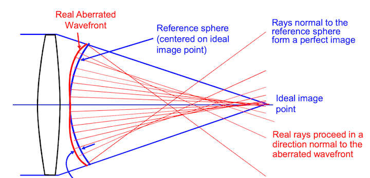
When calculating the wavefront error, the reference sphere is centered on the “expected” image location (usually the image surface location of the chief ray). It may be that a different reference sphere will fit the actual wavefront better. If the center of the better reference sphere is at a different axial location than the expected image location, there is a “focus error” in the wavefront. If the center of the better reference sphere is at a different lateral location than the expected image location, there is a “tilt error” in the wavefront
RMS Wavefront Error in Zemax
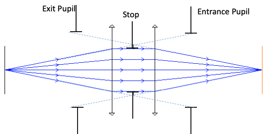
Ray trace programs will report “Wavefront Errors” at the Exit Pupil of a system. The errors are the difference between the actual wavefront and the ideal spherical wavefront converging on the image point. In a system with aberrations, rays from different positions in the exit pupil may miss the ideal image position by various amounts when they reach the image plane. This is known as “Transverse Ray Aberration”, or ‘TRA’.
Zemax does not normally propagate waves through an optical system but rather uses a geometric relationship between Ray errors and wavefront errors to calculate the wavefront error map. Since rays are always perpendicular to wavefronts, a wavefront tilt error (at some location in the pupil) corresponds directly to a Transverse Ray error (TRA) at the image plane. By tracing a number of rays through the pupil,and measuring the TRA of each, we can get the slope of σ; then by numerical integration, we can find the wavefront aberrations, σ.
Measuring Wavefront errors in real systems
There are different ways to measure the wavefront distortions introduced by an optical system. We can use interferometric methods, however these may be limited to the use of coherent light (like a laser). Shack-Hartmann wavefront sensors can work in incoherent and even broad-band light. A Shack-Hartmann wavefront sensor consists of an array of micro-lenses focusing portions of an incoming wavefront onto position-sensitive detectors.
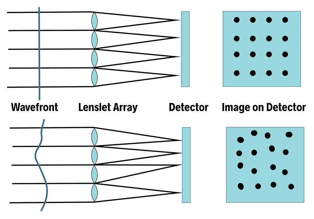
example of wavefront error
Shack–Hartmann sensors are used in astronomy to measure telescopes and in medicine to characterize eyes for corneal treatment of complex refractive errors
Источник
Pixel size issues
What should I do if the pixel size turned out to be wrong?В
If the error is small (say 1-2 %) and the resolution is not very high (3 Г…), you can specify the correct pixel size in the PostProcess job. This scales the resolution in the FSC curve. When the error is large, the presence of spherical aberration invalidates this approach. Continue reading.
You should not edit your STAR files because your current defocus values are fitted against the initial, slightly wrong pixel size. Also, you should not use “Manually set pixel size” in the Extraction job. It will make metadata inconsistent and break Bayesian Polishing. Thus, this option was removed in RELION 3.1.
Cs and the error in the pixel size
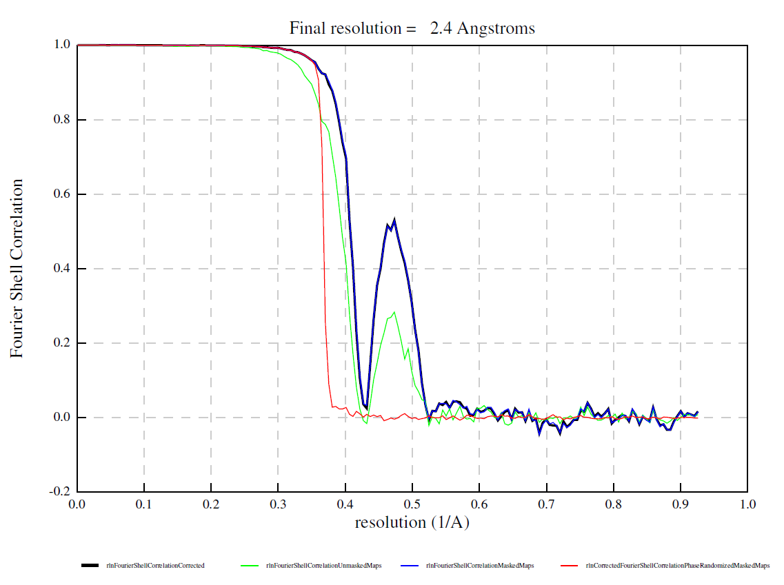
Recall that the phase shift due to defocus is proportional to the square of the wave number (i.e. inverse resolution), while that due to spherical aberration is proportional to the forth power of the wave number. At lower resolutions, the defocus term dominates and errors in the pixel size (i.e. errors in the wave number) can be absorbed into the defocus value fitted at the nominal pixel size. At higher resolution, however, the Cs term becomes significant. Since Cs is not fitted but given at the correct pixel size, the error persists. As the two terms have the opposite sign, the errors sometimes cancel out at certain resolution shells, leading to a strange bump in the FSC curve. See an example below contributed from a user. Here the pixel size was off by about 6 % (truth: 0.51 Г…/px, nominal: 0.54 Г…/px).
Below is a theoretical consideration. Let’s consider a CTF at defocus 5000 Å, Cs 2.7 mm at 0.51 Å/px. This is shown in orange. If one thought the pixel size is 0.54 Å/px, the calculated CTF (blue) became quite off even at 5 Å (0.2).
![]()
However, the defocus is fitted (by CtfFind, followed by CtfRefine) at 0.54 Г…/px, the nominal pixel size. The defocus became 5526 Г…, absorbing the error in the pixel size. This is shown in blue. The fit is almost perfect up to about 3.3 Г…. In this region, you can update the pixel size in PostProcess. Beyond this point, the error from the Cs term starts to appear and the two curves go out of phase. This is why the FSC drops to zero. However, the two curves came into phase again at about 1.8 Г… (0.55)! This is why the FSC goes up again.
![]()
If you refine Cs and defocus simultaneously, the error in the pixel size is completely absorbed and the fit becomes perfect. Notice that the refined Cs is 3.39, which is 2.7 * (0.54 / 0.51)^4. Also note that the refined defocus 5606 Г… is 5000 * (0.54 / 0.51)^2.
![]()
In practice, one just needs to run CtfRefine twice: first with Estimate 4th order aberrations to refine Cs, followed by another run for defocus. Note that rlnSphericalAberration remains the same. The error in Cs is expressed in rlnEvenZernike . You should never edit the pixel size in the STAR file!
Now everything is consistent at the nominal pixel size of 0.54 Г…/px. In PostProcess, one should specify 0.51 Г…/px to re-scale the resolution and the header of the output map.
How can I merge datasets with different pixel sizes?В
First of all: it is very common that one of your datasets is significantly better (i.e. thinner ice) than the others and merging many datasets does not improve resolution. First process datasets individually and then merge the most promising two. If it improves the resolution, merge the third dataset. Combining millions of bad particles simply because you have them is a very bad idea and waste of storage and computational time!
From RELION 3.1, you can refine particles with different pixel sizes and/or box sizes. Suppose you want to join two particle STAR files. First, make sure they have different rlnOpticsGroupName . For example:
Then use JoinStar. The result should look like:
Note that the dataset2’s rlnOpticsGroup has been re-numbered to 2.
If two datasets came from different detectors and/or had very different pixel sizes, you might want to apply MTF correction during refinement. To do this, add two more columns: rlnMtfFileName to specify the MTF STAR file (the path is relative to the project directory) and rlnMicrographOriginalPixelSize to specify the detector pixel size (i.e. before down-sampling during extraction).
Refine this combined dataset. For a reference and mask, you must use the pixel size and box size of the first optics group (or use —trust_ref_size option). The output pixel size and the box size will be the same as the input reference map. After refinement, run CtfRefine with Estimate anisotropic magnification: Yes . This will refine the relative pixel size difference between two datasets. In the above example, the nominal difference is 10 %, but it might be actually 9.4 %, for example. Then run Refine3D again. The absolute pixel size of the output can drift a bit. It needs to be calibrated against atomic models.
For Polishing, do NOT merge MotionCorr STAR files. First, run Polishing on one of the MotionCorr STAR files with run_data.star that contains all particles. This will process and write only particles from micrographs present in the given MotionCorr STAR file. Repeat this for the other MotionCorr STAR files. Finally, join two shiny.star files from the two jobs. The —only_group option is not the right way to do Polishing on combined datasets.
How can I estimate the absolute pixel size of a map?В
Experimentally and ideally, one can use diffraction from calibration standards.
Computationally, one can compare the map and a refined atomic model. However, if the model has been refined against the same map, the model might have been biased towards the map. Also note that bond and angle RMSDs are not always reliable when restraints are too strong.
If you are sure that (Cs_<mbox>) given by the microscope manufacturer is accurate, which is often the case, AND the acceleration voltage is also accurate, you can optimize the pixel size such that the apparent Cs fitted at the pixel size becomes (Cs_<mbox>) .
First, find out the (Z_4^0) coefficient. This is the 7th number in rlnEvenZernike . The contribution of the spherical aberration to the argument of the CTF’s sine function is (1/2 pi lambda^3 k^4 Cs) , where k is the wave-number and О» is the relativistic wavelength of the electron (0.0196 Г… for 300 kV and 0.0251 Г… for 200 kV). (Z_4^0 = 6k^4 — 6k^2 + 1) . By comparing the (k^4) term, we find the correction to the Cs is (12 Z_4^0 / (pi lambda^3)) . Note that (-6k^2 + 1) terms are cancelled by the lower-order Zernike coefficients and can be ignored. Thus,
(10^<-7>) is to convert Cs from Г… to mm. (Cs_<mbox>) is what you used in CTFFIND (e.g. 2.7 mm for Titan and Talos).
Examples
In RELION 3.1, relion_refine (Refine3D, Class3D, MultiBody) stretches, shrinks, pads and/or crops input particles so that the output has the same nominal pixel size and the box size as the input reference. Let’s study what happens in various cases.
One optics group
Suppose your optics group says 1.00 Г…/px. If the header of your reference also says 1.00 Г…/px, particles are used without any stretching or shrinking. The output remains 1.00 Г…/px.
Let’s assume that the nominal pixel size of 1.00 Å/px turns out slightly off and the real pixel size is 0.98 Å/px. As discussed above, you should never change the pixel size in the optics group table, since all CTF parameters, coordinates and trajectories are consistent with the nominal pixel size of 1.00 Å/px. When the header of your reference is 1.00 Å/px, the output map header says 1.00 Å/px, but it is actually 0.98 Å/px. Thus, you should specify 0.98 Å/px in PostProcess. The post-processed map will have 0.98 Å/px in the header and the X-axis of the FSC curve will be also consistent with 0.98 Å/px.
You must not use this 0.98 Г…/px map from PostProcess in future Refine3D/MultiBody/Class3D jobs. Otherwise, relion_refine stretches nominal 1.00 Г…/px particles into 0.98 Г…/px. Thus, the output map will have the nominal pixel size of 0.98 Г…/px but the actual pixel size will be 0.98 * 0.98 / 1.00 = 0.96 Г…/px!
Multiple optics groups
Suppose your have two optics groups, one at 1.00 Г…/px and the other at 0.95 Г…/px. If the header of your reference is 1.00 Г…/px, the particles in the first group are used without any stretching or shrinking, while those from the second group are shrunk to match 1.00 Г…/px. The output map is at 1.00 Г…/px.
Let’s assume that the real pixel size of the first group is exactly at 1.00 Å/px, while that of the second group is actually 0.90 Å/px. After stretching by the ratio between the nominal pixel size and the pixel size in the reference header, the true pixel size for the second group corresponds to 0.90 / 0.95 * 1.00 = 0.947 Å/px. Thus, the reconstruction is a mixture of particles at 1.00 Å/px and 0.947 Å/px. Depending on the number and signal-to-noise ratio of particles in each group, the real pixel size of the output can be any value between 0.947 and 1.00 Å/px, while the output header says 1.00 Å/px.
Anisotropic magnification refinement in CtfRefine finds the relative pixel size differences between particles and the reference. Suppose the actual pixel size of the output from Refine3D is 0.99 Г…/px and there is no anistropic magnification. CtfRefine finds the particles in the first group look smaller in real space than expected and puts 0.9900 0 0 0.9900 in rlnMatrix00, 01, 10, 11 (0.9900 = 0.99 / (1.00 * 1.00 / 1.00)). The particles in the second group look larger in real space than expected and rlnMatrix00 to rlnMatrix11 will be 1.045 0 0 1.045 (= 0.99 / (0.90 / 0.95 * 1.00)).
Источник
Optical sizing of nanoparticles in thin films of nonabsorbing nanocolloids
Gesuri Morales-Luna and Augusto García-Valenzuela
Author Affiliations
Gesuri Morales-Luna 1, * and Augusto García-Valenzuela 2
1 Escuela de Ingeniería y Ciencias, Tecnológico de Monterrey, Av. Eugenio Garza Sada 2501, Apartado Postal 64849, Monterrey, N.L., Mexico
2 Instituto de Ciencias Aplicadas y Tecnología, Universidad Nacional Autónoma de México, Apartado Postal 70-186, Ciudad de México 04510, Mexico
ORCID
| Gesuri Morales-Luna |  https://orcid.org/0000-0002-9323-3094 https://orcid.org/0000-0002-9323-3094 |
Your library or personal account may give you access
- Get PDF
- Share
- Share with Facebook
- Tweet This
- Post on reddit
- Share with LinkedIn
- Add to CiteULike
- Add to Mendeley
- Add to BibSonomy
- Get Citation
Abstract
We study an optical method to infer the size of nanoparticles in a thin film of a dilute nonabsorbing nanocolloid. It is based on determining the contribution of the nanoparticles to the complex effective refractive index of a suspension from reflectivity versus the angle of incidence curves in an internal reflection configuration. The method requires knowing only approximately the particles’ refractive index and volume fraction. The error margin in the refractive index used to illustrate this technique was 2%. The method is applicable to sizing nanoparticles from a few tens of nanometers to about 200 nm in radius and requires a small volume of the sample, in the range of a few microliters. The method could be used to sense nanoparticle aggregation and is suitable to be integrated into microfluidic devices.
© 2019 Optical Society of America
R. Márquez-Islas, C. Sánchez-Pérez, and A. García-Valenzuela
Appl. Opt. 54(31) 9082-9092 (2015)Arkadiusz Rudzki, Dean R. Evans, Gary Cook, and Wolfgang Haase
Appl. Opt. 52(22) E6-E14 (2013)H. Contreras-Tello and A. García-Valenzuela
Appl. Opt. 53(21) 4768-4778 (2014)Roberto Márquez-Islas and Augusto García-Valenzuela
Appl. Opt. 57(13) 3390-3394 (2018)Anays Acevedo-Barrera and Augusto Garcia-Valenzuela
Opt. Express 27(20) 28048-28061 (2019)References
You do not have subscription access to this journal. Citation lists with outbound citation links are available to subscribers only. You may subscribe either as an Optica member, or as an authorized user of your institution.
Contact your librarian or system administrator
or
Login to access Optica Member SubscriptionCited By
You do not have subscription access to this journal. Cited by links are available to subscribers only. You may subscribe either as an Optica member, or as an authorized user of your institution.
Contact your librarian or system administrator
or
Login to access Optica Member SubscriptionFigures (4)
You do not have subscription access to this journal. Figure files are available to subscribers only. You may subscribe either as an Optica member, or as an authorized user of your institution.
Contact your librarian or system administrator
or
Login to access Optica Member SubscriptionTables (1)
You do not have subscription access to this journal. Article tables are available to subscribers only. You may subscribe either as an Optica member, or as an authorized user of your institution.
Contact your librarian or system administrator
or
Login to access Optica Member SubscriptionEquations (5)
You do not have subscription access to this journal. Equations are available to subscribers only. You may subscribe either as an Optica member, or as an authorized user of your institution.
Contact your librarian or system administrator
or
Login to access Optica Member SubscriptionИсточник
Неисправности монетоприемников NRI G46; NRI Currenza
Не правильно выдает сдачу?
Для возобновления правильной работы монетоприемник нужно обнулить.
Порядок обнуления монетоприемника:
а) для версии монетоприемника NRI G46
Для обнуления счетчиков труб следует использовать встроенную клавиатуру монетоприемника (кнопки L, ML, MR, R). Чтобы имитировать выплату одной монеты из трубы, нажмите однократно соответствующую кнопку. Для обнуления счетчика каждой трубы нажмите на соответствующую кнопку и удерживайте ее не менее 4 секунд. Дождитесь окончания автоматической выплаты. Как только из трубы вылетела последняя монета, нажмите и удерживайте ту же кнопку для включения холостого хода, дайте монетоприемнику прокрутить вхолостую 5–6 оборотов. Эту операцию произведите последовательно для каждой трубы монетоприемника.
Важно: кнопку «+» не нажимать!
б) для версии монетоприемника NRI CURRENZA
Для обнуления счетчиков труб следует использовать встроенную клавиатуру (кнопки A, B, C, D, E, F). Чтобы имитировать выплату одной монеты из трубы, нажмите однократно соответствующую кнопку. Для обнуления счетчика трубы нажмите на кнопку и удерживайте ее не менее 4 секунд. Дождитесь окончания автоматической выплаты. Как только из трубы вылетела последняя монета, нажмите и удерживайте кнопку для включения холостого хода, дайте монетоприемнику прокрутить вхолостую 5–6 оборотов. Эту операцию произведите последовательно для каждой трубы монетоприемника.
Важно: кнопки «+», «MENU» не нажимать!
После обнуления перезагрузите весь автомат с помощью кнопки “ON/OFF” и, войдя в меню загрузки сдачи, загрузите монеты. В каждую трубу монетоприемника необходимо внести минимум по три монеты каждого номинала, только после этого он начнет отображать сумму сдачи на дисплее.
Не заполняет трубы до конца
Для возобновления правильной работы монетоприемник нужно обнулить.
Алгоритм обнуления монетоприемника подробно описан выше (пункт «Неправильно выдает сдачу»).
В случае, если операция не помогла, проверить индикацию монетоприемника. Левый светодиод должен гореть зеленым. Необходимо проверить остаток сдачи в меню «Загрузка сдачи». Счетчик должен быть равен нулю. Если счетчик нулю не равен, необходимо провести повторное обнуление, дать каждой трубе по 15 оборотов.
Если не помогло, разобрать монетоприемник, проверить на засор и сухой тряпочкой без ворса протереть датчики. Внимание, не применяйте никаких чистящих средств при чистке датчиков!
Инструкция по разборке монетоприемника есть ниже, в разделе «Не выдает монеты».
Возникает расхождение между суммой монет в монетоприемнике и в меню загрузка сдачи
Для возобновления правильной работы монетоприемник нужно обнулить.
Алгоритм обнуления монетоприемника подробно описан выше (пункт «Неправильно выдает сдачу»).
Не выдает монеты
Существует несколько возможных причин неисправности.
Для уточнения причины откройте денежный отсек и проверьте следующие параметры монетоприемника:
а) Если на монетоприемнике мигает красный диод, возможно, произошло засорение монетоприемника монетами.
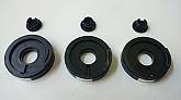
Для устранения неисправности необходимо открутить и поднять верхнюю крышку аппарата (см. соответствующий пункт Инструкции оператора), затем снять валидаторную головку монетоприемника (его верхнюю часть, через которую поступают монеты).
Чтобы снять валидаторную головку:
— на монетоприемнике NRI G46 необходимо, соблюдая осторожность, отверткой приподнять пластмассовую защелку (А), одновременно потянув на себя головку (B) (см. рис.). После снятия головки отсоедините ее от подведенного кабеля.
Для NRI G46
— на монетоприемнике NRI CURRENZA поднимите фиксатор, а затем снимите валидаторную головку движением на себя и в сторону.
Сняв валидаторную головку, аккуратно очистите ее монетный тракт и монетный тракт основания с механизмом выплаты сдачи от монет и посторонних предметов. Монетный тракт основания с механизмом выплаты сдачи расположен у задней стенки справа.
б) Если на монетоприемнике мигает желтый светодиод, это означает, что постоянно нажат рычаг возврата монет.
Проверьте работу рычага возврата монет. При плавном нажатии и отпускании рычага должно быть слышно срабатывание микро-выключателя. Отрегулируйте нажимную пластину механизма кнопки возврата аппарата.
в) Если не наполняется одна или несколько труб, причиной может быть западание флажка оптического датчика заполнения соответствующей трубы.
Флажок расположен внутри трубы, в верхней ее части. Снимите головку монетоприемника и обеспечьте свободный ход соответствующего флажка, либо удалите его.
г) Если монеты в одной или нескольких трубах не выдаются на сдачу, возможно, произошло заклинивание монеты в механизме выплаты сдачи.
Для устранения заклинивания необходимо нажать на кнопку, соответствующую данной трубе и, не сильно постукивая по нижней части основания с механизмом выплаты сдачи, попробовать устранить заклинивание.
Источник
Ремонт монетоприемника NRI Currenza
Монетоприемник NRI CURRENZA не имеет равных по скорости приема монет а
так же по емкости кассеты — 6 труб, и соответственно сложен по кострукции.
Отремонтировать его своими силами бывает не так просто. Мы осуществляем
ремонт, продажу, гарантийное и послегарантийное обслуживание
монетников NRI CURRENZA любой сложности, в кртчайшие сроки и обычно
в Вашем присутствии. Если неисправность можно диагностировать сразу то время
ремонта занимает от 30 до 60 минут.


Мы чиним платы, меняем моторы, датчики приема монет, производим замену
корпусных деталей и меняем прошивку монетоприемника на новую.


В монетоприемнике NRI Currenza установлены 6 клапанов и соответственно
столько же электромагнитных катушек которые через несколько лет работы
необходимо разобрать и почистить иначе монетник потеряет былую
скорость приема а так же возможны ошибки в раскладке монет по трубам.
Чистка с разборкой занимает около 30 минут, стоимость чистки 500р.


Механизм выдачи монет имеет три высокоскоростных мотора с установленной
на каждом платой драйверов и датчиками положения шестерни. Каждый мотор
монетника работает на две трубы и в случае застревания монеты в какой либо
из труб блокируются обе трубы. В большинстве случаев возможен ремонт
механизма выдачи монет без замены двигателей.
Время ремонта занимает около часа, стоимость 1000р.


Монетоприемник NRI Currenza выпускается в нескольких модификациях WHITE,
GREEN и BLUE. Первая модель не имеет даже клавиатуры и самая бюджетная,
вторая GREEN оборудована кнопками каждая из которых соответствует своей
трубе и номиналу монеты а так же клавишу с помощью которой возможна
загрузка монет непосредственно через монетоприемник а не через меню аппарата.
Наиболее полноценная модель Currenza Blue имеет по мимо клавиатуры
еще и дисплей с помощью которого можно менять настройки, просматривать
статистику, сделать диагностику и многое другое. Замена клавиатуры или
дисплея занимает до одного часа, стоимость работы 1000р.


Ремонт или замена сенсоров приема монет которых у Currenza три, обычно
требуется не ранее чем через 3 года работы монетоприемника. В некоторых
случаях датчики отлично равботают и после 6 лет эксплуатации монетника.
Мы призводим замену датчиков за 30 минут, стоимость работ 1000р.


Кассета с шестью трубами состоит из множества мелких деталей и
конструктивно сложна. Если Вы случайно повредили кассету Вашего
NRI Currenza то мы сможем быстро восстановить ее работоспособность установив
поврежденные детали. Так же у нас возможна замена труб и изменение
конфигурации монетника на любую из доступных.
Источник
Peak-to-Valley (PV) and Root-Mean-Square (RMS) are two common parameters used to measure the difference between an ideal optic surface to the actual optic surface. Historically the PV is used more often than RMS but RMS is a much better method for measuring the feat of an optic. Neither one of them are perfect parameters to fully calculate the optics’ performance.
PV is the measurement of the height difference between the highest point and the lowest point on the surface of the optic. In an ideal world, the PV will solve the worst cases of the optics’ performance at the eyes of optics designer. This is only true if there is low order of aberration or large size features on the optics. It also assumes that the measurements are precise and optics surface is noise free.
In reality, the surface of an optic has imperfections that are within less than 1mm to aperture. The measurement is also processed with instrument having vast difference of MTF (modular transfer function) and noise level. Each manufacturer has its own proprietary “measuring method” to mask the actual measurements. It basically interpolates the standard parameters to something unknown to designers, professionals or vendors. This practice from manufacturers will be primarily based on the interpolator’s knowledge of optical performance and can quickly go out of control.
It is quite common to see cost and manufacturability to be determined purely upon the value of PV. Most will demand a 1/10 wave PV optics without specifying the testing condition and with minimum budget. This will result in an unworkable project or over priced component or reinterpreted specification by vendor. It is nearly impossible to get absolute 1/10 wave PV optics in the manufacturing process.
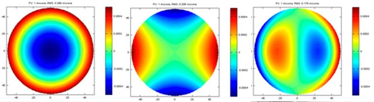
Plots of 1 micron PV for basic terms of aberration and its corresponding RMS are shown below. As you can see, the RMS is noticeably different for each basic term of aberration. Considering the similarity of alignment error in each system, the performance impact of each term is all relative to the ability of aligning specific error out at the final system.
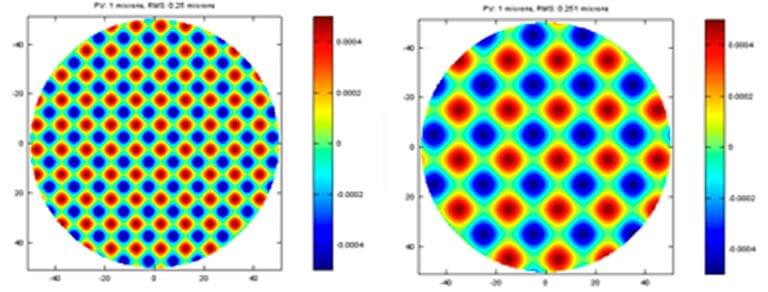
Modern optics is often made by sub-aperture polishing with computer controller motions. This creates another challenge when creating the specification of an optic. Due to the nature of sub-aperture polishing, the error on the surface is often showing as cyclical form. Two different frequency of this kind error is shown plots with the same 1-micron PV. If you can align most of the basic aberration in your system, this cyclical form error is not typically compensated in optical system. You notice that the PV and RMS are essential same or similar to the basic aberration terms, which is partially correctable at the system.
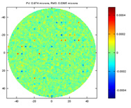
In well fabricated optics, the error mostly contains small but frequent imperfections plus occasional spikes of large but localized error. A simulated error of this kind is presented below. While the PV is still close to 1 microns, the RMS is much smaller than the errors shown previously. This is where the RMS really works while the PV completely fails to capture the quality of the optics.
The quality of optics should not be determined with just the numbers from PV or RMS. Contact Us for a free quote and consultation. With 20 years experience, we offer consulting service to help you find the specification you need for your optics.
JOHN FILHABER
When it comes to high-performance optical systems, mid-spatial-frequency (MSF) errors can affect applications in a wide variety of ways. For example, when present in cinematography optics, MSF errors can dramatically affect the quality of the «bokeh,» especially when the MSF is present on aspheres (bokeh is the esthetic quality of an out-of-focus blur). In high-resolution surveillance systems, MSF errors can degrade overall image contrast.
Yet, for many high-performance systems being deployed today, MSF errors are either trivialized or simply overlooked. Even when MSF concerns are identified, the modeling challenge for most designers can be daunting without specific knowledge of the manufacturing process. For example, while many opticians are familiar with the characteristic MSF «fingerprint» in their polishing process, they rarely isolate the data in such a way that designers can incorporate it in their tolerancing.
To understand the impact and causes of MSF errors, we first need to describe the surface in terms of its frequency content. To do this, we use Fourier analysis to «sort out» the surface by frequency content. The result is then plotted as a power-spectral-density (PSD) plot. The power in a specific frequency «bin» in units of l2l (l = length) is plotted against spatial frequency in units of l-1.
At the low-frequency end of the plot are errors typically described by terms such as figure, power, irregularity, or Zernike polynomial specifications. At the high-frequency end are errors usually described by surface-roughness specifications such as Ra (arithmetic average of the absolute values) and Rq (root-mean-square value). Errors with frequencies in between are variously called MSF, ripple, waviness, smoothness, or slope error. While definitions vary, for the audience in the theater or the analyst reviewing battle imagery to obtain the strongest possible image contrast, depth, and dimension, the entire spectrum of errors must be considered by designers and manufacturers to understand and control performance of an optical system.
Figure 1 shows a PSD plot from a 3D optical-profiler (Zygo Corporation’s NewView) measurement of a diamond-turned surface. The calculated root-mean-square (RMS) error and the Ra of the surface at 1.8 nm and 1.3 nm are consistent with a 2.0 nm RMS roughness requirement. The PSD of the surface in the y (long) direction gives a more-detailed picture of the surface. The frequencies shown correspond to periods from 100 μm to 0.5 μm. There is a clear peak at 250 mm that corresponds to the diamond-tool feed rate of 4 μm per turn.
Impact of MSF on performance
Surface errors affect optical performance in different ways depending on their frequency content, operational wavelength, and location in a system. The performance impact of an error at a given frequency is a way to define the boundaries between the low, medium, and high spatial frequencies. Low-spatial-frequency errors—such as power, astigmatism, and coma and those described by Zernike polynomials through Z36—broaden the point-spread function (PSF) of a system. High-spatial-frequency errors scatter light at high angles either out of a system or into a system. MSF errors impact a different regime, scattering light out of the core of the PSF without changing its shape, but at angles small enough to illuminate the focal plane—resulting in effects like hazing, subtle reduction of the range of shades in dark areas of an image, or uneven texture in out-of-focus portions of an image. Figure 2 shows a surface with and without MSF errors and their impact on the PSF.
A detailed analysis of MSF error’s influence on system performance is beyond the scope of this article but can be found in the references at the end of the article. A few useful oversimplifications will provide some visibility into the scale and form of the impact. Parameters such as modulation transfer function (MTF) depend, among other things, on the angle into which the MSF error scatters the light. An estimate of the scatter angle, θ, can be had from the grating equation, θ = arcsin (λ/d — sin θi), where θi is the incident angle, d is the period of the grating (or in this case, of the surface error), and λ is the operating wavelength of the system. From this we can see that light will be diffracted away from the core of a PSF by an angle that is a function of the wavelength of the system, and spatial frequency (f = 1/d) of the grating, or in our case, the error.
In the case of regular errors like diamond-turning tool marks or the print-through of the structure of a lightweighted mirror, this approximation works quite well. For more random errors, the scattering pattern is not regular, but the grating equation still gives good guidance as to where the light will wind up. In the example in Fig. 1, the tool marks from the diamond tool would scatter light at an angle of about 7° in the visible. In a wide-field imaging system, this surface, if uncorrected, would put objectionable rainbows around bright objects that a pitch-polished surface would not.
The high-frequency limit of MSF may be set by the point where the scattering angle approaches the aperture of the system. The regime beyond this limit is commonly described as surface roughness. At that point, the impact on the system is global and contributes to the veiling glare of a system.
The reduction of the intensity of the core of the PSF relative to the peak intensity of the diffraction-limited PSF is called the Strehl ratio, or simply Strehl. For small errors, the impact on Strehl can be approximated by the equation:
A good approximation of the total integrated scatter (TIS) is TIS ≈ (4πσ/λ)2. From this it is immediately apparent that a surface in an extreme-ultraviolet (EUV) lithography system operating at 13.5 nm would scatter 200X more energy than an equivalent surface used in an immersion lithography system at 193 nm.
MSF in design
For the most-demanding applications, the optical designer’s goal—defining and specifying high-quality, manufacturable optical assemblies—has been hampered by a failure to acknowledge the consequences of MSF when moving away from full-aperture pitch polishing to fast, modern machined optics. Taking note of MSF within the design and specifying the surface tolerance for the frequency are now important.
During the design of an optical system or element, MSF errors are usually considered in tolerancing since the design wavefront is controlled with low-frequency terms such as radius and a handful of coefficients for general-asphere terms or Zernike polynomials. In this sense, spatial frequencies higher than those that are represented by the first Zernikes (approximately 5 cycles across an imaging aperture) may be a reasonable lower limit to MSF.
Optical-design software includes capabilities for modeling scatter in a system and its impact on MTF and other parameters. Code V (Synopsys; Mountain View, CA) and Zemax (Radiant Zemax; Redmond, WA), for instance, include several scattering functions that can be attached to a surface and then evaluated using nonsequential ray-tracing and image-analysis tools.
The size of the subaperture that is illuminated by a point on an object is a key parameter when estimating error contributions to system performance. As an example, a lens with a clear aperture of 50 mm and MSF errors with 0.2/mm range will behave differently depending on the size of the illuminated subaperture. If this lens is at the pupil, the entire surface will contribute a wavefront aberration of approximately 10 cycles across the aperture. Light will be predominantly scattered on the order of 30 arcsec from the core of the image while the PSF will remain intact. At a window near the focal plane where the imaging bundle may be 2 mm in diameter, the spatial periods are a few times larger than the subaperture; the main consequence would be tilt or a shift of the image contributing to distortion.
Specifying MSF
The specifications of the elements in an optical system should completely guarantee that the systems assembled from these components will meet all of the user’s requirements. It is the design engineer’s first task to «flow down» the requirements to specifications that the manufacturer can understand, measure, and control. Indicating only the traditional radius, power, irregularity, and roughness specifications is clearly not enough to guarantee high performance from even a spherical surface. Point-spread function may be achieved, but Strehl, encircled energy, MTF, and flare will not be constrained.
To have the greatest degree of artistic control over the final image, editors and directors of photography are asking for better lens assemblies from manufacturers, but typically describe the effects qualitatively, because of a lack of exposure to specifications that affect these image features. Delivering the full range of the director of photography’s vision requires a much more detailed set of parameters than limiting resolution and MTF. Specifying the lens elements themselves needs more detail as well, since a cinematography lens with poor MSF but otherwise good power, figure, and roughness will produce distracting patterns in the out-of-focus portions of an image and apparent loss of contrast as light scattered from bright objects in the field obscures details in shadows that the eye would otherwise be able to detect.
ISO 10110-8, the International Organization for Standardization’s optics and photonics drawing standards pertaining to surface texture (roughness and waviness), provides several methods and standard notation for specifying limits on MSF content. The simplest is RMS waviness, or Wq. The drawing callout is simply:
where Wq is the RMS waviness between C and D, the upper and lower limits of the spatial bandwidth. Including sampling length is an improvement over a one-number RMS specification, but still falls short of constraining the relative frequency content of the MSF errors. Because the error in the evaluation range is integrated and compared to a single value, a surface whose frequency content is smooth may have the same RMS value as one that has a strong but narrow peak. This will often lead to undesirable artifacts in performance, ranging from reduced MTF to ghost images from very regular periodic defects.
ISO 10110-8 also defines a more-complete specification using the PSD that allows control of the frequency content of the MSF errors as well. The PSD drawing callout sets a two-term upper limit for the PSD with the equation: PSD(f) = A/fB, where A is the height of the line and B is the slope (as before, C and D are the lower and upper limits of the spatial bandwidth):
In the event that no spatial bandwidth is specified, it is assumed to be 0.08 mm to 2.5 mm.
Manufacturing implications
Computer control and a small tool-contact area are key components of high-end optical manufacturing (especially for aspheres) and also the key contributors to the MSF fingerprint that they leave behind. With any computer-controlled polishing (CCP) method including small tool, ion-beam polishing (IBF), and magnetorheological finishing (MRF), special care and control of MSF errors is fundamental.
An example of MSF control in manufacturing a high-performance asphere is shown in Fig. 3. The PSD plot shows excellent performance across a dynamic range spanning six orders of magnitude.
Figure 4 shows the surface map of another part before and after MSF errors are corrected. Removing MSF errors from the figuring process is challenging, because in the same way that CCP figuring produces MSF errors, smoothing MSF errors can produce low-frequency figure errors.
MSF errors are not the realm of aspheres alone. MSF is of little concern on systems with all spherical lenses that are polished with full-aperture pitch tools. Small tool-contact areas, however, leave small-period errors behind. Automated, flexible, and high-volume spherical-lens production equipment has forced us to rewrite specifications to control regular and irregular patterns that are residuals of the tools and control errors in the equipment used.
Measuring MSF
Complete measurement of a surface from low-frequency to high-frequency errors requires a suite of instrumentation to determine the full range of surface features that influence performance in the many regimes in which a system is evaluated. The test equipment used must have a sampling bandwidth and instrument transfer function (ITF = [PSDmeasured/PSDideal]1/2) sufficient to detect and accurately characterize the errors being measured.
The bandwidth and the ITF of an instrument are driven by a few factors—namely, sampling and optical design. Sampling is simply the density of data points that are projected on a surface. This sets a lower limit for spatial periods that can be measured across an aperture. For instance, a conventional large-aperture Fizeau interferometer with a 1K × 1K camera measuring a 1-m-diameter mirror will sample the surface with 1 mm spacing. The spatial-frequency cutoff for this system is driven by the Nyquist limit—in this case twice the sampling period, or 2 mm. The optical design and quality of the optics in the instrument set a further limit on the ITF since a large blur spot will mask all smaller features regardless of the number of pixels in the camera.
Building an instrument with excellent frequency response places a high bar on design, algorithm, and fabrication technologies. Figure 5 shows the measured ITF of a DynaFiz interferometer with a 1200 × 1200 camera through its range of zooms on a 100 mm part. At all zooms, the ½ Nyquist ITF remains 90% of the theoretical (90%) limit.
Typically, a Fizeau interferometer will be used for the lowest-frequency measurements and a scanning white-light interferometer (SWLI) microscope will be used for the high-frequency measurements. MSF errors may span most of the measuring range of both instruments.
An SWLI microscope is typically used to continue the measurement spectrum from the high-frequency limit of the Fizeau to the limit of the roughness specification. For example, the NewView 7300 optical profiler, with a 1K × 1K camera, a 2.5X objective, and a 1X zoom tube, would overlap the sampling range in the previous example and extend the Nyquist-limited sampling down to 8 μm periods. Switching to a 20X objective will lower the Nyquist sampling limit to 1 μm. The diffraction limit of this objective is 0.7 μm, so in this case the Nyquist sampling limit will be twice that, or 1.4 μm.
Custom metrology instruments are sometimes required to support extreme performance programs. Figure 6 shows the measured ITF of a custom SWLI system developed for semiconductor lithography. The customer needed to verify optics with a 0.1 nm RMS (4–400 cycles/mm) specification. The flowed-down instrument requirement of ITF greater than 70% at 400 cycles/mm was surpassed by the system.
Measurement control and analysis software can collect and immediately display the data as a PSD and make it available for other types of analysis. The entire frequency range of data from several instruments and measurements can be combined into a single plot that allows direct evaluation of imaging performance over the entire frequency range of errors on a surface. In one example (see Fig. 6), data from a large-aperture interferometer is combined with two measurements from a SWLI microscope to provide a PSD spanning four decades of spatial periods from 20 mm to 1 μm.
The old saw, «Beauty is in the eye of the beholder,» certainly applies to MSF considerations. What would be perceived as MSF for meter-class optics could easily be interpreted as a low-order error for smaller components. Similarly, artifacts like diamond-turning marks on a longwave-infrared lens might be deemed «smooth» for its application and wavelength, but would be judged unacceptable in another usage. As we strive for optimal results in our diverse optical assemblies, it is important for all stakeholders in an optical element to become knowledgeable about MSF considerations. The designer needs to properly specify optics. The manufacturer must ensure these specifications can be met. And to measure them, the metrologist must understand the true capabilities of the applicable instruments.
ACKNOWLEDGEMENT
Zygo, NewView, and DynaFiz are trademarks of Zygo Corporation.
REFERENCES
1. ISO 10110-8:2010(E), Optics and photonics — Preparation of drawings for optical elements and systems — Part 8: Surface texture; roughness and waviness 4.3.
2. P. Croce and L. Prod’Homme, Opt. Comm., 20–24 (October 1980).
3. J. M. Tamkin, T. D. Milster, and W. Dallas, Appl. Opt., 49, 25, 4825 (September 2010).
4. J. M. Tamkin, W. J. Dallas, and T. D. Milster, Appl. Opt., 49, 25, 4814 (September 1, 2010).
5. R. N. Youngworth and B. D. Stone, Appl. Opt., 39, 13, 2198 (May 1, 2000).
6. «High performance Fizeau and scanning white-light interferometers for mid-spatial frequency optical testing of free-form optics,» Leslie L. Deck and Chris Evans, Zygo Corporation, Laurel Brook Road, Middlefield, CT 06455.
7. «Advanced Metrology Tools Applied for Lithography Optics Fabrication and Testing,» Masaru Ohtsuka Production Engineering Research Lab, Canon Inc., Optical Fabrication & Testing (October 11, 2006).
John Filhaber is Director of Special Projects at Zygo Corporation, Middlefield, CT; e-mail: jfilhaber@zygo.com;www.zygo.com.
New Results
doi: https://doi.org/10.1101/285692
Abstract
Optical mapping is a unique system that is capable of producing high-resolution, high-throughput genomic map data that gives information about the structure of a genome [21]. Recently it has been used for scaffolding contigs and assembly validation for large-scale sequencing projects, including the maize [32], goat [6], and amborella [4] genomes. However, a major impediment in the use of this data is the variety and quantity of errors in the raw optical mapping data, which are called Rmaps. The challenges associated with using Rmap data are analogous to dealing with insertions and deletions in the alignment of long reads. Moreover, they are arguably harder to tackle since the data is numerical and susceptible to inaccuracy. We develop cOMet to error correct Rmap data, which to the best of our knowledge is the only optical mapping error correction method. Our experimental results demonstrate that cOMet has high prevision and corrects 82.49% of insertion errors and 77.38% of deletion errors in Rmap data generated from the E. coli K-12 reference genome. Out of the deletion errors corrected, 98.26% are true errors. Similarly, out of the insertion errors corrected, 82.19% are true errors. It also successfully scales to large genomes, improving the quality of 78% and 99% of the Rmaps in the plum and goat genomes, respectively. Lastly, we show the utility of error correction by demonstrating how it improves the assembly of Rmap data. Error corrected Rmap data results in an assembly that is more contiguous, and covers a larger fraction of the genome.
Introduction
In 1993 Schwartz et al. developed optical mapping, a system for creating an ordered, genome-wide, high-resolution restriction map of a given organism’s genome. Since this initial development, genome-wide optical maps have found numerous applications including discovering structural variations and rearrangements [24], scaffolding and validating contigs for several large sequencing projects [7, 9, 4], and detecting misassembled regions in draft genomes [16]. Thus, optical mapping has assisted in the assembly of a variety of species–including various prokaryote species [18, 29, 30], rice [31], maize [32], mouse [5], goat [7], parrot [9], and amborella trichopoda [4]. The raw optical mapping data is generated by a biological experiment in which large DNA molecules cling to the surface of a microscope slide using electrostatic charge and are digested with one or more restriction enzymes. The restriction enzymes cut the DNA molecule at occurrences of the enzyme’s recognition sequence, forming a number of DNA fragments. The fragments formed by digestion are painted with a fluorescent dye, to allow visibility under laser light and a CCD camera. Computer vision algorithms then estimate fragment length from consolidated intensity of fluorescent dye and apparent distance between fragment ends.
The resulting data from an experiment are in the form of an ordered series of fragment lengths [33]. The data for each single molecule produced by the system is called an Rmap. Rmap data has a number of errors due to the experimental conditions and system limitations. In an optical mapping experiment, it is unlikely to achieve perfectly uniform fluorescent staining.
This leads to an erroneous estimation of fragment sizes. Also, restriction enzymes often fail to digest all occurrences of their recognition sequence across the DNA molecule. This manifests as missing restriction sites. Additionally, due to the fragile nature of DNA, additional breaks can incorrectly appear as restriction sites. Lastly, the limitations of the imaging component of the optical mapping system and the propensity for the DNA to ball up at the ends introduces more sizing error for smaller fragments. Interested readers will find more details about the causes of these errors in Valouev et al. [26] and Li et al. [12]. Because of all these experimental conditions, Rmap data generated through optical mapping experiment has insertion (added cut sites) and deletion (missed cut sites) errors along with fragment sizing errors.
In most applications of optical map data, the Rmaps need to be assembled into a genome wide optical map. This is because the single molecule maps need redundant sampling to overcome the presence of the aforementioned errors, and because single molecule maps only span on the order of 500 Kbp [26]. The first step of this assembly process involves finding pairwise alignments amongst the Rmaps. In order to accomplish this, the challenge of dealing with missing fragment sizes has to be overcome. This challenge is analogous to dealing with insertions and deletions in the alignment of long reads [2]— in fact, it is arguably harder since the data is numerical. At present, the only non-proprietary algorithmic method for pairwise alignment of Rmaps is the dynamic programming based method of Valouev et al. [26] which runs in O(α×β) time where α and β are the number of fragments in the two Rmaps being aligned. To align an optical map dataset containing n Rmaps, the complexity becomes O(n2 × 𝓁2) where 𝓁 is the average size of an Rmap.
This method is inherently computationally intensive but if the error rate of the data could be improved then non-dynamic-programming based methods that are orders of magnitude faster such as Twin [15], OMBlast [10], and Maligner [13] could be used for alignment. This would greatly improve the time required to assemble Rmap data. Thus, we present cOMet in order to address this need. To the best of our knowledge, it is the first Rmap error correction method. Our experimental results demonstrate that cOMet has high precision and corrects 82.49% of insertion errors and 77.38% of deletion errors in Rmap data generated from the E.coli K-12 reference genome. Out of the deletion errors corrected, 98.26% are true errors. Similarly, out of the insertion errors corrected, 82.19% are true errors. Furthermore we show that the assembly of Rmaps is more contiguous and covers a larger fraction of the genome if the Rmaps are first error corrected. It also successfully scales to large genomes, improving the quality of 78% and 99% of the Rmaps in the plum and goat genome, respectively.
Background
From a computer science perspective, optical mapping can be seen as a process that takes in two strings: a nucleotide sequence Si[1, n] and a restriction sequence B[1, b], and produces an array (string) of integers Ri[1, m]. The array Ri is an Rmap corresponding to Si and contains the string-lengths between cuts produced by B on Si. Formally, Ri is defined as follows: Ri[j] = y – x where y represents the location(starting index) of jth occurrence of B in Si and x represents the location of (j – 1)th occurrence of B in Si and Ri[1] = y – 1 and Ri[m] = n – x. For example, say we have B = act and Si = atacttactggactactaaact. The locations of B in Si are as follows: 3,7,12,15,20. Then Ri will be represented as Ri = 2, 4, 5, 3, 5, 2. The size of an Rmap denotes the number of fragments in that Rmap. Therefore the size of Ri is 6.
We note that millions of Rmaps are produced for a single genome since optical mapping is performed on many cells of the organism and each cell provides thousands of Rmaps. The Rmaps can be assembled to produce a genome wide optical map. This is analogous to next generation shotgun sequencing where Rmaps are analogous to reads and a genome-wide optical map is analogous to the assembled whole genome.
There are three types of errors that can occur in optical mapping: (1) missing cut sites which are caused by an enzyme not cleaving at a specific site, (2) additional cut sites which can occur due to random DNA breakage and (3) inaccuracy in the fragment size due to the inability of the system to accurately estimate the fragment size. Continuing again with the example above, a more representative example Rmap would include these errors, such as  .
.
The error rates of optical maps depends on the platform used for generating the maps. A recent paper by Li et al. [12] studied the error rates of optical maps produced by the Irys system from BioNano Genomics. According to their study, a missing cut site type of error i.e., error type (1) happens when a restriction site is incompletely digested by the enzyme and causes two flanking fragments to merge into one large fragment. The probability of complete digestion of a restriction site can be modeled as a Bernoulli trial whose probability of success is a function of the size of the two flanking fragments. Additional cut sites i.e., error type (2) results from random breaks of the DNA molecule. The number of false cuts per unit length of DNA follows a Poisson distribution. The inaccuracy of the fragment sizes, i.e., error type (3), is modeled using a Laplace distribution. If the observed and actual size of a fragment are ok and rk respectively, then the sizing error is defined as sk = ok/rk and

where µ and β -the parameters of the laplace distribution -are functions of rk. In practice, when aligning a pair of Rmaps, one should allow for twice the error rate of a single Rmap since each Rmap will deviate from the genomic map by the above parameters.
Valouev et al. [26] provides a dynamic programming algorithm for pairwise alignment, which generates a score for every possible alignment between two Rmaps and returns the alignment which achieves the highest score, which is referred to as the S-score. It is computed within a standard dynamic programming framework, similar to Smith-Waterman alignment [23]. The scoring function is based on a probabilistic model built on the following assumptions: the fragment sizes follow an exponential distribution, the restriction sites follow an independent Bernoulli process, the number of false cuts in a given genomic length is a Poisson process, and the sizing error follows a normal distribution with mean zero and variance following a linear function of the true size. Lastly, a different sizing error function is used for fragments less than 4 kbp in length since they do not converge to the defined normal distribution. The score of an alignment is calculated as the sum of two functions; one function that estimates and scores the sizing error, and a second that predicts and scores the presence of additional and/or missing cut sites between the fragments. The S-score will be used later in this paper to evaluate the error correction process.
Methods
Given a set of n Rmaps R = {R1, .., Rn} our method aims to detect and correct all errors in R by considering each Ri ∈ R and finding a set of Rmaps that originate from the same part of the genome as Ri. This step is performed heuristically in order to avoid aligning every pair of Rmaps in R.
Preprocessing
Our first step is to remove the first and last fragments from each Rmap in R. These fragments have one of their edges sheared by artifacts of the DNA prep process (preceding the optical mapping process) and not by restriction enzymes. Unless removed, they can misguide alignment between two Rmaps during the error correction process. In addition, short Rmaps, i.e., those that have less than 10 fragments, are removed at this stage since any Rmap that contains less than 10 fragments is typically deemed too small for analysis even in consensus maps [1]. Next, the data is quantized so that a given genomic fragment is represented by the same value across multiple Rmaps despite the noise. Our quantization method assigns a unique value to a range of fragment sizes by dividing each fragment size by a fixed integer, denoted as b, and rounding to the nearest integer. For example, if an Rmap Ri = {36, 13, 15, 20, 16, 5, 21, 17} is quantized using b = 3 then the quantized Rmap will be  .Say another Rmap, Rj = {17, 23, 34, 12, 14, 21, 14, 5} has overlap with Ri; however, due to noise in the data, this relation is not apparent. By quantizing Rj using the same b = 3 we get
  . This allows us to uncover a region (in this case {4, 5, 7, 5}) which is common to both the Rmaps. It should be noted that in some cases, a fragment may have different values across two Rmaps even after quantization (for example the fragment values 36 from Ri and 34 from Rj are quantized to 12 and 11 respectively). The quantized data is used to find the set of related Rmaps as explained in the next section.
The setting of parameter b depends on the amount of sizing error in the optical map data. With zero sizing error b can be set at 1. As sizing error increases, the value of b is increased accordingly. If the value of b is too small, we are not be able to uncover relations between overlapping Rmaps and if the value is too large then unrelated Rmaps have common regions in their quantized states — which makes them appear related. Considering the error rate of optical maps from BioNano genomics, the default value of b = 4000.
Finding Related Rmaps
We refer to two Rmaps as related if their corresponding errorfree Rmaps originate from overlapping regions of the genome. Next, we define a k-mer as a string of k consecutive fragments from a (quantized) Rmap. For example if we have the Rmap R = {3, 3, 5, 2, 6, 5, 5, 1} and k=4 then the following k-mers can be extracted from R: (3,3,5,2), (3,5,2,6), (5,2,6,5), (2,6,5,5) and (6,5,5,1). In order to avoid aligning all pairs of Rmaps to find the related Rmaps, we use the number of common k-mers to discriminate between pairs of Rmaps that are related and those that are not. To accomplish this eficiently, we first extract all unique k-mers in each quantized Rmap, and construct a hash table storing each unique k-mer as a key and the list of Rmaps containing an occurrence of that k-mer as the value. We call this the k-mer index. Next, we consider each Ri in R and use the k-mer index to identify the set of Rmaps that have m or more k-mers in common with Ri. Unfortunately, this set, although it contains all related Rmaps, it also likely contains Rmaps that are not related to Ri. Therefore, we filter this set of Rmaps using a simple heuristic that tries to match each Rmap in this set with Ri in order to ascertain if it is related to Ri. The heuristic traverses through two Rmaps (Ri and one Rmap from the set, say Rj) attempting to match subsets of the fragments from each until it either reaches the end of one Rmap or it fails to match the fragments. We start the traversal from the first matching k-mer between Ri and Rj. We denote the position of the next fragment to be matched in Ri and Rj as x and y, respectively, and assume that each fragment prior to these positions is matched. Next, we consider all combinations of matching the fragments at positions x, x + 1 and x + 2 of Ri with fragments at positions y, y + 1 and y + 2 of Rj. We evaluate the cost of each combination based on the difference in the total size of fragments from Ri and Rj. That is ∀α, β = [0, 2],

where Ri[g] and Rj[h] denotes the g-th and h-th fragments of Ri and Rj respectively. We select the combination with the least cost; if there exists a tie, we select the match that has the least number of added or missing cut sites (That is, the combination with the least value of α + β). If this selected match leads to a cost that is greater than a specified threshold (which was set to 25% of the larger sized fragment in practice), then we conclude that there is not a match at these positions and return that Ri and Rj are unrelated. Otherwise, we increment x and y accordingly and move onto the next fragments. If this heuristic continues until the last fragment of either Ri or Rj is reached then we return that Ri and Rj are related. Using this heuristic we filter out the Rmaps that were deemed to be related based on the number of k-mers in common with Ri but are infact unrelated to Ri.
The setting of parameters k and m are correlated. If the value of k is increased, that makes the k-mers more specific, hence, the value of m is lowered. On the other hand, if the value of k is reduced, then we increase the value of m. The value of k is increased when there are fewer insertion and deletion errors and decreased otherwise. The default values are k = 4 and m = 1.
Rmap Alignment
Next, for each Ri in R, we use the alignment method of Valouev et al. [26] to find the S-score of all pairwise alignments between Ri and each Rmap in its set of related rmaps. The Rmaps that have an alignment score, i.e., S-score less than a defined threshold (which we denote as St), are removed from the set of related Rmaps and the alignments of the remaining Rmaps are stored in a multiple alignment grid, denoted as Ai. This grid is a two-dimensional array of integer pairs, where the number of rows is equal to the number of remaining Rmaps in the set of related Rmaps of Ri and the number of columns is equal to the number of fragments in Ri. An element of this array, Ai[j, k] stores an integer pair in the form of (x, y) representing that x fragments of Ri, (which includes the k-th fragment of Ri) matches to y fragments of Rj in the optimal alignment between Ri and Rj. Figure 1 illustrates an example of Ai. The first fragment of Ri does not match with any fragment of Rj and therefore, (0, 0) is stored at this position. Fragments 2, 5, 6, 8 and 9 of Ri each matches with one fragment of Rj, e.g., 1, 3, 4, 7 and 8, respectively. To represent these matches, we store a (1,1) in 2nd, 5th, 6th, 8th and 9th column of row j. Fragments 3 and 4 of Ri match with one fragment of Rj, i.e., the 2nd fragment. To represent this, we store (2,1) in Ai[j, 3] and Ai[j, 4]. Fragment 7 of Ri matches with two fragments of Rj, i.e., the 5th and 6th fragments. To represent this, we store (1,2) in Ai[j, 7]. Fragments 10 and 11 of Ri match with two fragments of Rj, i.e., the 9th and 10th fragments. To represent this, we store (2,2) in positions Ai[j, 10] and Ai[j, 11]. Finally, fragments 12 and 13 match with three fragments of Rj, i.e., fragments 11, 12 and 13. In this case, we store (2,3) in positions Ai[j, 12] and Ai[j, 13].

- Download figure
- Open in new tab
Figure 1.
An alignment between Ri and Rj as given by Valouev et al. [26] and its corresponding entry in the multiple alignment grid Ai. Each column of Ai represents one fragment from Ri and each row represents one Rmap from its’ set of related Rmaps. The fragment sizes are in Kbp.
The setting of parameter St controls the number of Rmaps that are included in the multiple-alignment-grid of an Rmap. If we increase the value of St, fewer Rmaps will be added to the grid — but the ones included will be of higher quality (i.e. have greater overlap with the Rmap under consideration). The default value for the parameter St = 8. We show in the experiment section how we select this value.
Error Correcting Using the Consensus
The multiple alignment grid is used to find the consensus grid, denoted as Ci, for Rmap Ri. The grid Ci is a one-dimensional array of integer pairs with size equal to the number of fragments in Ri. The grid is constructed for each Ri in R by iterating through each column of Ai and finding the most frequent integer pair, breaking ties arbitrarily. The most frequent integerpair is stored at each position of Ci if the frequency is above a given threshold d; otherwise, (0,0) is stored. Figure 2 illustrates the construction of a consensus grid from an alignment grid. The type of error in each fragment of Ri can be identified using Ci[k] = (x, y) as follows: if x and y are equal then a sizing error occurs at the k-th fragment of Ri, otherwise, if x is greater than y then an additional cut site exists, and lastly, if x is less than y then a missing cut site exists. Next, we use Ci and Ai to correct these errors in Ri. For each fragment of Ri, we consider the consensus stored at the corresponding position of Ci, identify the positions in the corresponding column of Ai that are equal to it, and replace the fragment of Ri with the mean total fragment size computed using the values at those positions in Ai. If Ci is equal to (0,0) at any position then the fragment at that position in Ri remains unchanged since it implies that there is no definitive result about the type of error in that position. In addition, if consecutive positions in Ci are discordant then the fragments in those positions in Ri also remains unchanged. For example, if there is a (2,1) consensus at some position of Ci, then we expect the preceding or successive position to also have a (2,1) consensus. However, if this is not the case, then we do not error correct those fragments since the consensus is discordant at those positions. Figure 2 shows this error correction. As it is illustrated, to error correct the second fragment of Ri, we compute the average of the matched fragments from related Rmaps 2, 3, 4, 5 and 6 and replace the second fragment of Ri with that value as shown in Figure 2. Similarly, to correct the third fragment in this example, we identify that (2,1) is in the consensus, which implies that majority of the related Rmaps are such that two fragments of Ri match with one fragment from the set of related Rmaps, and therefore, replace the third and fourth fragments with the average from the corresponding Rmaps and positions.

- Download figure
- Open in new tab
Figure 2.
Example of multiple alignment grid and consensus grid. The figure shows the multiple alignment grid Ai for an Rmap Ri and its consensus grid Ci. Each row of the multiple alignment grid represents the alignment of Ri with one of its related Rmaps while the columns represents the fragments of Ri. The figure also demonstrates error correction using the consensus grid, with the error corrected Rmap denoted as  . The fragment sizes are in Kbp. To demonstrate the error correction process for the 3rd, 4th and 5th fragments, we also include the fragments (in parentheses) to which they align. The error corrected fragment is the mean of the fragments from the corresponding positions which have the same alignment as the consensus. For example for the 5th fragment, the consensus is (1,1). Therefore the mean of the aligned fragments with (1,1) alignment i.e. 8.488, 8.132, 8.964 and 9.432 is the error-corrected value for the 5th fragment.
The threshold d determines the accuracy and precision of error correction. A high value of d improves precision but lowers accuracy as many fragments are left uncorrected. Similarly, low value of d improves accuracy but lowers precision. The default setting is d = 3.
Complexity
We define 𝓁 to be the length of the longest Rmap in R. Quantization of the Rmaps takes O(𝓁 × n) time. Constructing the k-mer index also takes O(𝓁 × n) time. The k-mer index stores the occurances of each quantized k-mer across all Rmaps. Let u be maximum frequency of a k-mer. That is, a k-mer occurs in max u Rmaps (in practice u << n). Then the complexity of finding related Rmaps from the k-mer index is O(n× 𝓁 × u). For each Rmap, the filtering heuristic runs in time linear to the size of the Rmap. Therefore, filtering the set of related Rmaps also takes linear O(𝓁 × n) time. The most expensive step is the pair-wise alignment which uses the Valouev aligner. As mentioned earlier, this aligner is based on DP and therefore has a O(𝓁2) time complexity to perform one pairwise alignment. If the maximum cardinality of the set of related Rmaps for any Rmap is v, then the total complexity of this step is bounded by O(n × v × 𝓁2). The value of v depends on the coverage of the optical map data. The alignment generated using Valouev et al. method is stored in the multiple alignment grid in constant time and it takes O(n × v × 𝓁) time to generate the consensus maps for n Rmaps and error correct them. Thus, the runtime of cOMet is O(n × v × 𝓁2).
Datasets
We perform experiments on both simulated and real data. For the real data, we used the Rmap data from the plum [28] and domestic goat [7] sequencing projects. These datasets were built on the OpGen mapping platform and are more error-prone. We also experimented on a human dataset [22] built on the new BioNano platform. This dataset is built using the latest optical mapping technology and has significantly better quality than the plum and goat genomes. The genome size and number of Rmaps for these species are shown in Tables 1 and 1.
Table 1.
Summary of the real and simulated data. Rmaps with less than 10 fragments were omitted from all the experiments. cOMet was ran on the remaining 2,504, 548,779 and 3,049,439 Rmaps for the E. coli, plum and goat genomes, respectively..
Table 2.
Summary of the real and simulated BioNano data. OM-Sim was used to simulate eight different BioNano datasets; each of which had varying error rates and thus, had a different number of Rmaps.
In addition, we simulated Rmap data from E. coli K-12 sub-str. MG 1655 as follows: first, the reference genome was copied 200 times and then uniformly distributed random loci were selected for each of these copies. These loci form the ends of single molecule that would undergo in silico digestion. Next, molecules smaller than 150 Kbp were discarded and the cleavage sites for the RsrII enzyme were then identified within each of these simulated molecules. This error free Rmap data is used for validating the output of our method. Lastly, deletion, insertion and sizing errors were incorporated into the errorfree Rmaps according to the error model discussed in Li et al. [12]. The error model was described earlier in the Background section. This simulation resulted in 2,505 Rmaps, containing 7,485 deletion and 554 insertion errors.
Lastly, we simulated optical map data from a simulation software called OMSim [14] that generates synthetic optical maps which mimics real Bionano Genomics data. The software takes two parameters as input: the False Positive Rate (FP), which is the number of additional cut sites erroneously inserted per 100kbp, and the False Negative Rate (FN), which is the percentage of times a cut site is missed. Using this method, we simulated eight datasets of Rmaps from E. coli K-12 substr. MG 1655 using the restriction enzyme BspQI. The default FP and FN rates for BspQI are 1 and 15% respectively.
We generated additional datasets with the following error rates (FP,FN) : (0.5,15%), (1.0,15%), (2.0,15%),(5.0,15%), (1.0,5%), (1.0,25%),(2.0,5%) and (2.0,25%).
Experiments and Discussion
We performed all experiments on Intel E5-2698v3 processors with 192 GB of RAM running 64-bit Linux. The input parameters to cOMet include: b (quantization bucket size), k (k-mer value), m (the number of k-mers needed to be conserved between two Rmaps) and d (the minimum number of Rmaps required to form consensus at a position). The default parameters are b=4000, k=4, m=1 and d=3, and led to the best result across all datasets.
Determining the value of St
The setting of the parameter St depends on the sensitivity of the Valouev aligner. If the alignment score between two Rmaps is less than St, then the aligned Rmaps are deemed to be unrelated. We say an Rmap, Rs is overlapping with an Rmap, Rt if at least 50% of Rs overlaps with Rt. That is, either the first half or the second half of Rs is entirely and exactly (exact fragment matches) contained in Rt
We carried out the following experiment to determine the optimum setting for St. From the set of simulated error-free Rmaps, we computed the set of overlapping Rmaps for each Rmap. We denote this set as related Rmaps. Then we used the Valouev aligner to score all pairwise wise alignments between the simulated Rmaps (with errors added) and plot the scores in form of a histogram which is shown in Figure 3. The percentage of related Rmaps with S-score less than 8 is 6.06%. Hence we choose the setting of St = 8.

- Download figure
- Open in new tab
Figure 3.
Distribution of S-scores of Rmap alignments between related Rmaps and unrelated Rmaps. The percentage of Related Rmaps with S-score less than 8 is 6.06%. Therefore we choose St = 8.
Experiments with our Simulated Data
The cOMet error correction was ran on the simulated E. coli data. The corrected Rmaps were then aligned to the error-free Rmaps to determine the number of corrected insertions and deletions. The results of this experiment are shown in Table 4. To determine the quality of error correction, we computed the true positive rate (TPR), which is the ratio between the number of insertion (or deletion) errors that cOMet correctly identified and removed and the number of insertion (deletion) errors, and the false positive rate (FPR), which is the ratio between the number of insertion (or deletion) errors that cOMet incorrectly identified and removed, and the total number of fragments not containing an insertion (deletion) error. The TPR is 82.49% and 77.38% with respect to the number of corrected insertions and deletion errors; whereas, the FPR is 0.21% and 0.25% with respect to the number of corrected insertions and deletion errors. This demonstrates the high accuracy of the correction made by cOMet. Our method also has high precision. Out of the deletion errors corrected, 98.26% are true errors. Similarly, out of the insertion errors corrected, 82.19% are true errors.
Additionally, for each corrected Rmap we computed the alignment S-score of both the original Rmap and the corrected Rmap with the error-free Rmap. We found that for 96.5% of the Rmaps, the S-scores improved after error correction. In other words, cOMet brought 96.5% Rmaps closer to their error-free state. The mean S-score before error-correction was 44.91 and it improved by 14.03% to 51.30 after error correction. For 17.5% of the Rmaps, (415 Rmaps) the S-score improved by more than ten. Lastly, we mention that the error correction was achieved in 241 CPU seconds and using 79.54 MB of memory.
To demonstrate the importance of error correction, we assembled the Rmaps before and after error correction using the Valouev assembler [25]. Table 3 summarizes the results of this experiment. We assembled the uncorrected data into five assembled optical maps and the error-corrected data into two assembled optical maps. The N50 statistic of the assembly increased from 1,242 Kbp for the uncorrected data to 3,348 Kbp for the corrected data. Next, we aligned each assembled map to the genome-wide (error-free) optical map using the Valouev aligner in order to locate their positions on the genome and calculate the percentage of the genome that was covered by at least one of the assembled maps. The genome fraction covered by the five assembled maps from the uncorrected Rmaps was 80%; while the genome fraction covered by the two assembled maps from the corrected Rmaps was 82%. Moreover, the assembled maps from the uncorrected data had 47 insertion and deletion errors when aligned to the reference while the error corrected data had only 34 such errors. In order to further contextualize these results, we assemble the error-free Rmap dataset and summarize this assembly in Table 3.
Table 3.
Assembly results of Uncorrected Rmaps, Corrected Rmaps and Error-free Rmaps using the Valouev assembler. The Rmaps are simulated from the E. coli genome. Each assembled map is aligned to the reference genome-wide (error-free) optical map using the Valouev aligner. The genome-wide optical map contains 383 fragments.
Experiments with OMSim Data
To present the robustness of our method and its applicability across datasets, we conducted experiments on synthetic data from an optical map simulating software called OMSim [14]. As described in Section Datasets, we generated eight datasets of synthetic optical maps by varying the insertion and deletion error rates.
In the first experiment, we fixed the False Negative rate at 15% and varied the False Positive rate between 0.5, 1.0, 2.0 and 5.0 respectively. For each of the four datasets, we align each Rmap (using the Valouev aligner) before and after error correction to the reference optical map obtained using the same restriction enzyme and report the percent of Rmaps whose align-ment S-score increased after error correction and the mean in-crease in the S-score. We note that for each Rmap, the aligner returns the highest scored alignment and the score represents how closely the Rmap aligns to the reference genome-wide optical map. Table 6 summarizes the results from this experiment. We observe that the eficiency of error-correction improves as the FP rate is initially increased. When the FP rate reaches a high value of 5, the eficiency of error-correction drops. The mean S-score improves by more than 9 (∼ 10%) when the FP rate is reasonable.
In the second experiment, we first fix the False Positive rate at 1.0 and vary the False Negative rate between 5%, 15% and 25%. We then fix the False Positive rate at 2 and vary the false negative rate between 5%, 15% and 25%. We report the same results as the previous experiment. Table 7 shows the results. Similar to the previous experiment, we find that the eficiency of error correction improves as the FN rate increases from 5% to 25%. The error correction improves the quality of a high percentage of Rmaps (> 70%) for all values of parameters.
Experiments with Real Data
Table 5 summaries the results of running cOMet on the plum and goat datasets. The plum and goat datasets do not contain error-free Rmaps. Therefore, we are restricted to reporting the number of corrections made and the improvement to the S-score. In order to compute the S-score before and after error correction, we generated an in silico digested genome-wide optical map from the reference genome and aligned both the uncorrected and corrected Rmap to the genome-wide optical map. If it aligned to multiple positions then we considered the alignment position where the corrected Rmap aligned with greatest S-score, and considered the difference in the S-score when the uncorrected and corrected Rmap aligned to that position. However, we note that this process is error prone because of the fragmented nature of the draft genomes and possible misassemblies present in the genomes. We observed that the S-score after error correction improved for 78% of the plum Rmaps and 99% of the goat Rmaps. Figures 4 and 5 show the histograms of the distribution of S-scores, before and after error correction. For the plum genome, the mean S-score improved from 8.60 before error correction, to 14.72 after error correction (a 71% improvement in the score) while for the goat genome, it improved from 9.38 before correction to 16.97 after correction (a 80.92% improvement in the score).
Table 4.
Results on the data simulated from E.coli K-12 MG 1655. The data was simulated according the algorithm described in Datasets. This simulation resulted in 2,505 Rmaps, containing 7,485 deletion and 554 insertion errors.
Table 5.
Results on the Rmap data of plum and goat genomes. Peak memory was measured as the maximum resident set size as reported by the operating system with suficient RAM to avoid paging. Running time is the user process time, also reported by the operating system.
Table 6.
Table showing the eficiency of error correction when the False Positive rate is varied. The False Negative rate is fixed at 15%.
Table 7.
Table showing the eficiency of error correction when the False Negative rate is varied.

- Download figure
- Open in new tab
Figure 4.
Alignment scores of Rmaps from plum genome with the reference optical-map. Before error correction, the S-score had a mean of 8.6 with standard deviation 6.49. After error correction, the mean S-score improved to 14.72, with standard deviation 6.72.

- Download figure
- Open in new tab
Figure 5.
Alignment scores of rmaps from goat genome with the reference optical-map. The mean and standard deviation of the S-scores before error correction were 9.38 and 6.54, respectively. After error correction, the mean S-score improved to 16.97 with a standard deviation of 6.21.

- Download figure
- Open in new tab
Figure 6.
Distribution of Rmap lengths whose S-score increased after error correction. The Rmaps are simulated from the Ecoli K-12 substr. MG 1655 as explained in the text.

- Download figure
- Open in new tab
Figure 7.
Distribution of fragment sizes of Rmaps whose S-score increased after error correction. The Rmaps are simulated from the Ecoli K-12 substr. MG 1655 as explained in the text.
We also measured the genome coverage, i.e. the fraction of the genome covered by at least one Rmap, for both the original Rmaps and the corrected Rmaps as follows. First we aligned all Rmaps to the genome-wide optical map and then picked the best alignment for each original Rmap and each corrected Rmap. Based on these alignments we then computed the fraction of the genome covered by at least one original Rmap and the fraction of the genome covered by at least one corrected Rmap. On the goat genome the genome coverage was 73.08% before correction and it increased to 84.56% after correction. The increase in genome coverage shows that our method is able to correct Rmaps from across the genome. Furthermore it shows that even if Rmaps could not originally be reliably aligned to some regions of the genome, our method is sensitive enough to recover similar Rmaps from these regions and thus after correction the fraction of the genome covered by aligned Rmaps is higher. For the plum, the genome coverage dropped negligibly from 99.01% before error correction to 98.85% after error correction(which is less than 1% of the genome size).
In addition, as shown in Table 5, the running time and peak memory usage was recorded for the plum and goat genome. Although these experiments have significant running times, (7.4 and 105.7 CPU days for plum and goat, respectively) these figures are not prohibitive given that this computation can easily be parallelized since the error correction process for each Rmap is independent. For example, we ran the goat genome on 20 machines and thus, it required a total of 126.84 hours for all Rmaps to be corrected. In addition, we note that error correction of a dataset will likely only be done once for any dataset so 5.2 human days for a large genome is not unreasonable. Lastly, the peak memory usage was 12.20 GB and 113.56 GB, for plum and goat, respectively, and thus, cOMet is able to run on any modern server.
Next, we ran experiments on the human dataset. Again, since we do not possess the error free Rmaps corresponding to the raw Rmaps for this dataset, we follow a similar evaluation method as in the previous experiments. We performed our evaluation on a in silico digested human reference genome (Gen-Bank assembly accession: GCA_000001405.15, Genome Reference Consortium Human Build 38) using BspQI, which was the restriction enzyme that was used for generating the Rmap data. cOMet improves the S-score of 74.78% of the RMaps. The average S-score improves from 85.96 before error correction to after error correction.
Conclusion
Error correction of high-throughput sequencing data has become an imperative pre-processing step in genome assembly since 2008 when Chaisson and Pevzner showed the dramatic improvement it can have on the quality of the assembly [3, 8, 20]. For example, after error correction the contig N50 size of an assembly of Rhodabacter sphaeroides improved from 233 bp to 7,793 bp using the same assembler [20]. Due to this inarguable benefit on genome assembly, many methods have been developed for error correction of sequence reads, including BFC [11], Coral [19], EULER [17, 3] and Reptile [27]. Un-fortunately, even though there has been a massive effort into error correction of sequence data, there currently does not exist a publicly released method for error correction of Rmap data—a method that would likely improve the quality of genome-wide optical map assemblies, and allow such assemblies to be computed with greater eficiency.
In this paper, we presented cOMet, an error correction method for Rmap data, and demonstrate that it corrects and improves the quality of a high percentage of Rmaps in both the simulated and real datasets. As previously discussed, Rmap data is subject to high error rates. In addition to insertion and deletion errors, they contain sizing errors which necessitates the use of dynamic programming algorithm for pairwise alignment, and subsequently, assembly. By correcting a significant number of errors in Rmap data, cOMet can make it possible to use faster alignment methods [15, 10, 13], and explore the development of more eficient Rmap assembly algorithms.
Availability of Supporting Data
The optical mapping data for plum and goat is publicly available and can be accessed from their respective manuscripts. The simulated data for E.coli is provided in the github repository along with the python scripts used to generate it.
Supplementary material
In Figure 6 We show the distribution of lengths of Rmaps whose S-score increases after error correction. From the distribution we can tell that our method is able to error correct Rmaps of all sizes. We also show the distribution of fragment sizes from Rmaps whose score increases after error correction in Figure 7.
Acknowledgements
KM, DW, MM and CB were funded by the National Science Foundation (1618814) and LS was funded by Academy of Finland (grants 284598 (CoECGR), 308030, and 314170).
Footnotes
-
↵* cboucher{at}cise.ufl.edu
References
- 1.↵
Bradnam KR, et al. Assemblathon 2: Evaluating de novo methods of genome assembly in three vertebrate species. GigaScience 2013;2(1):1–31.
- 2.↵
Chaisson MJ, Tesler G. Mapping single molecule sequencing reads using basic local alignment with successive refinement (BLASR): application and theory. BMC Bioinformatics 2012;p. 238.
- 3.↵
Chaisson MJ, Brinza D, Pevzner PA. De novo fragment assembly with short mate-paired reads: Does the read length matter? Genome Res 2009;19(2):336–346.
- 4.↵
Chamala S, et al. Assembly and Validation of the Genome of the Nonmodel Basal Angiosperm Amborella. Science 2013;342(6165):1516–1517.
- 5.↵
Church DM, et al. Lineage-Specific Biology Revealed by a Finished Genome Assembly of the Mouse. PLoS Biology 2009;7(5):e1000112.#x002B;.
- 6.↵
Dong Y, et al. Sequencing and Automated Whole-Genome Optical Mapping of the Genome of a Domestic Goat. Nature Biotechnology 2013;31(2):136–141.
- 7.↵
Dong Y, et al., Sequencing and automated whole-genome optical mapping of the genome of a domestic goat (Capra hircus). Nature Biotechnol.; 2013.
- 8.↵
Ekblom R, Wolf JBW. A field guide to whole-genome sequencing, assembly and annotation. Evolutionary Applications 2014;7(9):1026–1042.
- 9.↵
Ganapathy G, et al. De novo high-coverage sequencing and annotated assemblies of the budgerigar genome. GigaScience 2014;3:11.
- 10.↵
Leung AKY, et al. OMBlast: alignment tool for optical mapping using a seed-and-extend approach. Bioinformatics 2016;p. btw620.
- 11.↵
Li H. BFC: correcting Illumina sequencing errors. Bioin formatics 2015;31(17):2885.
- 12.↵
Li M, et al. Towards a More Accurate Error Model for Bio-Nano Optical Maps. In: ISBRA 2016;. p. 67–79.
- 13.↵
Mendelowitz LM, et al. Maligner: a fast ordered restriction map aligner. Bioinformatics 2016;32(7):1016–1022.
- 14.↵
Miclotte G, Plaisance S, Rombauts S, Van de Peer Y, Audenaert P, Fostier J. OMSim: a simulator for optical map data. Bioinformatics 2017; p. 2740–2742.
- 15.↵
Muggli MD, Puglisi SJ, Boucher C. In: Eficient indexed alignment of contigs to optical maps; 2014. p. 68–81.
- 16.↵
Muggli MD, Puglisi SJ, Ronen R, Boucher C. Misassembly detection using paired-end sequence reads and optical mapping data. Bioinformatics 2015;31(12):i80–i88.
- 17.↵
Pevzner PA, Tang H, Waterman MS. An Eulerian Path Approach to DNA Fragment Assembly. Proceedings of the National Academy of Sciences 2001;98(17):9748–9753.
- 18.↵
Reslewic S, et al. Whole-Genome Shotgun Optical Mapping of Rhodospirillum Rubrum. Appl Environ Microbiol 2005;71(9):5511–5522.
- 19.↵
Salmela L, Schröder J. Correcting errors in short reads by multiple alignments. Bioinformatics 2011;27(11):1455–1461.
- 20.↵
Salzberg SL, et al. GAGE: A critical evaluation of 1. genome assemblies and assembly algorithms. Genome Res 2012;22(3):557–567.
- 21.↵
Schwartz DC, et al. Ordered Restriction Maps of Saccharomyces Cerevisiae Chromosomes Constructed by Optical Mapping. Science 1993;262:110–114.
- 22.↵
Shi L, et al. Long-read sequencing and de novo assembly of a Chinese genome. Nature Communications 2016 Jun;.
- 23.↵
Smith TF, Waterman MS. Identification of common molecular subsequences. J Mol Biol 1981;147(1):195 –197.
- 24.↵
Teague B, et al. High-Resolution Human Genome Structure by Single-Molecule Analysis. Proc Natl Acad Sci USA 2010;107(24):10848–10853.
- 25.↵
Valouev A, Schwartz DC, Zhou S, Waterman MS. An algorithm for assembly of ordered restriction maps from single DNA molecules. Proc Natl Acad Sci USA 2006;103(43):15770–15775.
- 26.↵
Valouev A, et al. Alignment of optical maps. J Comp Biol 2006;13(2):442–462.
- 27.↵
Yang X, Dorman KS, Aluru S. Reptile: representative tiling for short read error correction. Bioinformatics 2010;26(20):2526.
- 28.↵
Zhang Q, et al., Genomic data of the plum (Prunus mume). GigaScience Database; 2014.
- 29.↵
Zhou S, et al. A Whole-Genome Shotgun Optical Map of Yersinia pestis Strain KIM. Appl Environ Microbiol 2002;68(12):6321–6331.
- 30.↵
Zhou S, et al. Shotgun Optical Mapping of the Entire Leishmania major Friedlin Genome. Mol Biochem Parasitol 2004;138(1):97–106.
- 31.↵
Zhou S, et al. Validation of Rice Genome Sequence by Optical Mapping. BMC Genomics 2007;8(1):278.
- 32.↵
Zhou S, et al. A Single Molecule Scaffold for the Maize Genome. PLoS Genetics 2009 11;5:e1000711.
- 33.↵
Zhou S, Herschleb J, Schwartz DC. A single molecule system for whole genome analysis. Perspectives in Bioanalysis 2007;2:265–300.
As mentioned in several articles in this blog, aberrations are of great relevance when designing an optical system. The objective being to design a system that creates a “good image”. However, there are different metrics to evaluate what is a “good image”. Most of the time, a customer won’t express their image quality requirements in terms such as MTF or ray aberration plots. However, they know what they want the optical system to do. It is up to the optical engineer to translate those needs into a numerical specification. Some aberration measurement techniques are better for some applications than for others. For example, for long-range targets where the object is essentially a point source like in a telescope, RMS wavefront error might be an appropriate choice for system evaluation.
RMS wavefront error is a way to measure wavefront aberration. Basically, we compare the real wavefront with a perfect spherical wavefront. We are not going to derive the equation to physically calculate the RMS wavefront error. Here we will just say that the RMS wavefront error is given by a square root of the difference between the average of squared wavefront deviations minus the square of average wavefront deviation. The RMS value expresses statistical deviation from the perfect reference sphere, averaged over the entire wavefront.
When calculating the wavefront error, the reference sphere is centered on the “expected” image location (usually the image surface location of the chief ray). It may be that a different reference sphere will fit the actual wavefront better. If the center of the better reference sphere is at a different axial location than the expected image location, there is a “focus error” in the wavefront. If the center of the better reference sphere is at a different lateral location than the expected image location, there is a “tilt error” in the wavefront
RMS Wavefront Error in Zemax
Ray trace programs will report “Wavefront Errors” at the Exit Pupil of a system. The errors are the difference between the actual wavefront and the ideal spherical wavefront converging on the image point. In a system with aberrations, rays from different positions in the exit pupil may miss the ideal image position by various amounts when they reach the image plane. This is known as “Transverse Ray Aberration”, or ‘TRA’.
Zemax does not normally propagate waves through an optical system but rather uses a geometric relationship between Ray errors and wavefront errors to calculate the wavefront error map. Since rays are always perpendicular to wavefronts, a wavefront tilt error (at some location in the pupil) corresponds directly to a Transverse Ray error (TRA) at the image plane. By tracing a number of rays through the pupil,and measuring the TRA of each, we can get the slope of σ; then by numerical integration, we can find the wavefront aberrations, σ.
Measuring Wavefront errors in real systems
There are different ways to measure the wavefront distortions introduced by an optical system. We can use interferometric methods, however these may be limited to the use of coherent light (like a laser). Shack-Hartmann wavefront sensors can work in incoherent and even broad-band light. A Shack-Hartmann wavefront sensor consists of an array of micro-lenses focusing portions of an incoming wavefront onto position-sensitive detectors.
example of wavefront error
Shack–Hartmann sensors are used in astronomy to measure telescopes and in medicine to characterize eyes for corneal treatment of complex refractive errors