Как найти систематическую ошибку - Исправление ошибок и поиск оптимальных решений проблем

Систематическая
погрешность,
в отличие от случайной, сохраняет свою
величину (и знак) во время эксперимента.
Систематические погрешности появляются
вследствие ограниченной точности
приборов, неучета внешних факторов и
т.д.

Обычно
основной вклад в систематическую
погрешность
дает погрешность, определяемая точность
приборов, которыми производят измерения.
Т.е. сколько бы раз мы не повторяли
измерения, точность полученного нами
результата не превысит точности,
обеспеченной характеристиками данного
прибора. Для обычных измерительных
инструментов (линейка, пружинные весы,
секундомер) в качестве абсолютной
систематической погрешности берется
половина шкалы деления прибора. Так в
рассматриваемом нами случае работы N
24 величина h’
может измеряться с точностью =0.05
см,
если линейка имеет миллиметровые
деления, и =0.5
см,
если только сантиметровые.

Систематические
погрешности электроизмерительных
приборов, выпускаемых промышленностью,
определяется их классом точности,
который обычно выражается в процентах.
Электроизмерительные приборы по степени
точности подразделяются на 8 основных
классов точности:0.05, 0.1, 0.2, 0.5, 1, 1.5, 2.5, 4.
Класс
точности
есть
величина, показывающая максимально
допустимую
относительную погрешность в процентах.
Если например прибор имеет класс
точности 2, то это означает, что его
максимальная относительная погрешность
при измерении, например тока, равна 2 %,
т.е.

где
—
верхний предел шкалы измерений амперметра.
При этом величина
(абсолютная погрешность в измерении
силы тока) будет равна

(6)

для
любых измерений силы тока на данном
амперметре. Так как ,
вычисленное по формуле (6), это максимально
допустимая данным прибором погрешность,
то обычно считают, что для определения
,
погрешность, определяемую классом
точности прибора, нужно разделить на
два. Т.е.

и
при этом
будет так же одинакова для всех измерений
на данном приборе. Однако, относительная
погрешность (в нашем случае

где
I—
показания прибора) будет тем меньше,
чем ближе значение измеряемой величины
к максимально возможному на данном
приборе. Следовательно, лучше выбирать
прибор так, чтобы стрелка прибора при
измерениях заходила за середину шкалы.

В
реальных опытах присутствуют как
систематические, так и случайные ошибки.
Пусть они характеризуются абсолютными
погрешностями
и .
Тогда суммарная погрешность опыта
находится по формуле

(7)

Из
формулы (7) видно, что если одна из этих
погрешностей мала, то ей можно пренебречь.
Например, пусть
в 2 раза больше ,
тогда

т.е.
с точностью до 12% =.
Таким образом, меньшая погрешность
почти ничего не добавляет к большей,
даже если она составляет половину от
нее. В том случае, если случайная ошибка
опытов хотя бы вдвое меньше систематической,
нет смысла производить многократные
измерения, так как полная погрешность
опыта при этом практически не уменьшается.
Достаточно произвести 2 — 3 измерения,
чтобы убедиться, что случайная ошибка
действительно мала.

В
случае рассматриваемой нами работы N
24 =0.26
см,
а
равна либо 0.05 см,
либо 0.5 см.
В этом случае

Как
видно, в первом случае можно пренебречь
,
а во втором .

Соседние файлы в папке физика

#
#
29.03.201687.04 Кб6mekh1.doc
#
#
#
#

Источник

Систематической погрешностью называется составляющая погрешности измерения, остающаяся постоянной или закономерно меняющаяся при повторных измерениях одной и той же величины. При этом предполагается, что систематические погрешности представляют собой определенную функцию неслучайных факторов, состав которых зависит от физических, конструкционных и технологических особенностей средств измерений, условий их применения, а также индивидуальных качеств наблюдателя. Сложные детерминированные закономерности, которым подчиняются систематические погрешности, определяются либо при создании средств измерений и комплектации измерительной аппаратуры, либо непосредственно при подготовке измерительного эксперимента и в процессе его проведения. Совершенствование методов измерения, использование высококачественных материалом, прогрессивная технология — все это позволяет на практике устранить систематические погрешности настолько, что при обработке результатов наблюдений с их наличием зачастую не приходится считаться.

Систематические погрешности принято классифицировать в зависимости от причин их возникновения и по характеру их проявления при измерениях.

В зависимости от причин возникновения рассматриваются четыре вида систематических погрешностей.

1. Погрешности метода, или теоретические погрешности, проистекающие от ошибочности или недостаточной разработки принятой теории метода измерений в целом или от допущенных упрощений при проведении измерений.

Погрешности метода возникают также при экстраполяции свойства, измеренного на ограниченной части некоторого объекта, на весь объект, если последний не обладает однородностью измеряемого свойства. Так, считая диаметр цилиндрического вала равным результату, полученному при измерении в одном сечении и в одном направлении, мы допускаем систематическую погрешность, полностью определяемую отклонениями формы исследуемого вала. При определении плотности вещества по измерениям массы и объема некоторой пробы возникает систематическая погрешность, если проба содержала некоторое количество примесей, а результат измерения принимается за характеристику данного вещества -вообще.

К погрешностям метода следует отнести также те погрешности, которые возникают вследствие влияния измерительной аппаратуры на измеряемые свойства объекта. Подобные явления возникают, например, при измерении длин, когда измерительное усилие используемых приборов достаточно велико, при регистрации быстропротекаюших процессов недостаточно быстродействующей аппаратурой, при измерениях температур жидкостными или газовыми термометрами и т.д.

2. Инструментальные погрешности, зависящие от погрешностей применяемых средств измерений.. Среди инструментальных погрешностей в отдельную группу выделяются погрешности схемы, не связанные с неточностью изготовления средств измерения и обязанные своим происхождением самой структурной схеме средств измерений. Исследование инструментальных погрешностей является предметом специальной дисциплины — теории точности измерительных устройств.

3. Погрешности, обусловленные неправильной установкой и взаимным расположением средств измерения, являющихся частью единого комплекса, несогласованностью их характеристик, влиянием внешних температурных, гравитационных, радиационных и других полей, нестабильностью источников питания, несогласованностью входных и выходных параметров электрических цепей приборов и т.д.

4. Личные погрешности, обусловленные индивидуальными особенностями наблюдателя. Такого рода погрешности вызываются, например, запаздыванием или опережением при регистрации сигнала, неправильным отсчетом десятых долей деления шкалы, асимметрией, возникающей при установке штриха посередине между двумя рисками.

По характеру своего поведения в процессе измерения систематические погрешности подразделяются на постоянные и переменные.

Постоянные систематические погрешности возникают, например, при неправильной установке начала отсчета, неправильной градуировке и юстировке средств измерения и остаются постоянными при всех повторных наблюдениях. Поэтому, если уж они возникли, их очень трудно обнаружить в результатах наблюдений.

Среди переменных систематических погрешностей принято выделять прогрессивные и периодические.

Прогрессивная погрешность возникает, например, при взвешивании, когда одно из коромысел весов находится ближе к источнику тепла, чем другое, поэтому быстрее нагревается и

удлиняется. Это приводит к систематическому сдвигу начала отсчета и к монотонному изменению показаний весов.

Периодическая погрешность присуща измерительным приборам с круговой шкалой, если ось вращения указателя не совпадает с осью шкалы.

Все остальные виды систематических погрешностей принято называть погрешностями, изменяющимися по сложному закону.

В тех случаях, когда при создании средств измерений, необходимых для данной измерительной установки, не удается устранить влияние систематических погрешностей, приходится специально организовывать измерительный процесс и осуществлять математическую обработку результатов. Методы борьбы с систематическими погрешностями заключаются в их обнаружении и последующем исключении путем полной или частичной компенсации. Основные трудности, часто непреодолимые, состоят именно в обнаружении систематических погрешностей, поэтому иногда приходится довольствоваться приближенным их анализом.

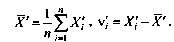
Способы обнаружения систематических погрешностей. Результаты наблюдений, полученные при наличии систематических погрешностей, будем называть неисправленными и в отличие от исправленных снабжать штрихами их обозначения (например, Х1, Х₂ и т.д.). Вычисленные в этих условиях средние арифметические значения и отклонения от результатов наблюдений будем также называть неисправленными и ставить штрихи у символов этих величин. Таким образом,

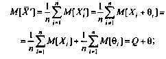
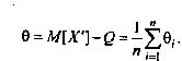
Поскольку неисправленные результаты наблюдений включают в себя систематические погрешности, сумму которых для каждого /-го наблюдения будем обозначать через 8., то их математическое ожидание не совпадает с истинным значением измеряемой величины и отличается от него на некоторую величину 0, называемую систематической погрешностью неисправленного среднего арифметического. Действительно,

Если систематические погрешности постоянны, т.е. 0_/ = 0, /=1,2, …, п, то неисправленные отклонения могут быть непосредственно использованы для оценки рассеивания ряда наблюдений. В противном случае необходимо предварительно исправить отдельные результаты измерений, введя в них так называемые поправки, равные систематическим погрешностям по величине и обратные им по знаку:

q = -Oi.

Таким образом, для нахождения исправленного среднего арифметического и оценки его рассеивания относительно истинного значения измеряемой величины необходимо обнаружить систематические погрешности и исключить их путем введения поправок или соответствующей каждому конкретному случаю организации самого измерения. Остановимся подробнее на некоторых способах обнаружения систематических погрешностей.

Постоянные систематические погрешности не влияют на значения случайных отклонений результатов наблюдений от средних арифметических, поэтому никакая математическая обработка результатов наблюдений не может привести к их обнаружению. Анализ таких погрешностей возможен только на основании некоторых априорных знаний об этих погрешностях, получаемых, например, при поверке средств измерений. Измеряемая величина при поверке обычно воспроизводится образцовой мерой, действительное значение которой известно. Поэтому разность между средним арифметическим результатов наблюдения и значением меры с точностью, определяемой погрешностью аттестации меры и случайными погрешностями измерения, равна искомой систематической погрешности.

Одним из наиболее действенных способов обнаружения систематических погрешностей в ряде результатов наблюдений является построение графика последовательности неисправленных значений случайных отклонений результатов наблюдений от средних арифметических.

Рассматриваемый способ обнаружения постоянных систематических погрешностей можно сформулировать следующим образом: если неисправленные отклонения результатов наблюдений резко изменяются при изменении условий наблюдений, то данные результаты содержат постоянную систематическую погрешность, зависящую от условий наблюдений.

Систематические погрешности являются детерминированными величинами, поэтому в принципе всегда могут быть вычислены и исключены из результатов измерений. После исключения систематических погрешностей получаем исправленные средние арифметические и исправленные отклонения результатов наблюдении, которые позволяют оценить степень рассеивания результатов.

Для исправления результатов наблюдений их складывают с поправками, равными систематическим погрешностям по величине и обратными им по знаку. Поправку определяют экспериментально при поверке приборов или в результате специальных исследований, обыкновенно с некоторой ограниченной точностью.

Поправки могут задаваться также в виде формул, по которым они вычисляются для каждого конкретного случая. Например, при измерениях и поверках с помощью образцовых манометров следует вводить поправки к их показаниям на местное значение ускорения свободного падения

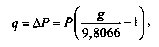
где Р — измеряемое давление.

Введением поправки устраняется влияние только одной вполне определенной систематической погрешности, поэтому в результаты измерения зачастую приходится вводить очень большое число поправок. При этом вследствие ограниченной точности определения поправок накапливаются случайные погрешности и дисперсия результата измерения увеличивается.

Систематическая погрешность, остающаяся после введения поправок на ее наиболее существенные составляющие включает в себя ряд элементарных составляющих, называемых неисключенными остатками систематической погрешности. К их числу относятся погрешности:

• определения поправок;

• зависящие от точности измерения влияющих величин, входящих в формулы для определения поправок;

• связанные с колебаниями влияющих величин (температуры окружающей среды, напряжения питания и т.д.).

Перечисленные погрешности малы, и поправки на них не вводятся.

Источник

Experimental techniques

Yanqiu Huang, … Zhixiang Cao, in Industrial Ventilation Design Guidebook (Second Edition), 2021

4.3.3.2 Measurement errors

The measurement errors are divided into two categories: systematic errors and random errors (OIML, 1978).

Systematic error is an error which, in the course of a number of measurements carried out under the same conditions of a given value and quantity, either remains constant in absolute value and sign, or varies according to definite law with changing conditions.

Random error varies in an unpredictable manner in absolute value and in sign when a large number of measurements of the same value of a quantity are made under essentially identical conditions.

The origins of the above two errors are different in cause and nature. A simple example is when the mass of a weight is less than its nominal value, a systematic error occurs, which is constant in absolute value and sign. This is a pure systematic error. A ventilation-related example is when the instrument factor of a Pitot-static tube, which defines the relationship between the measured pressure difference and the velocity, is incorrect, a systematic error occurs. On the other hand, if a Pitot-static tube is positioned manually in a duct in such a way that the tube tip is randomly on either side of the intended measurement point, a random error occurs. This way, different phenomena create different types of error. The (total) error of measurement usually is a combination of the above two types.

The question may be asked, that is, what is the reason for dividing the errors into two categories? The answer is the totally different way of dealing with these different types. Systematic error can be eliminated to a sufficient degree, whereas random error cannot. The following section shows how to deal with these errors.

Read full chapter

URL:

https://www.sciencedirect.com/science/article/pii/B9780128166734000043

EXPERIMENTAL TECHNIQUES

KAI SIREN, … PETER V. NIELSEN, in Industrial Ventilation Design Guidebook, 2001

12.3.3.11 Systematic Errors

Systematic error, as stated above, can be eliminated—not totally, but usually to a sufficient degree. This elimination process is called “calibration.” Calibration is simply a procedure where the result of measurement recorded by an instrument is compared with the measurement result of a standard. A standard is a measuring device intended to define, to represent physically, to conserve, or to reproduce the unit of measurement in order to transmit it to other measuring instruments by comparison.¹ There are several categories of standards, but, simplifying a little, a standard is an instrument with a very high accuracy and can for that reason be used as a reference for ordinary measuring instruments. The calibration itself is usually carried out by measuring the quantity over the whole range required and by defining either one correction factor for the whole range, for a constant systematic error, or a correction curve or equation for the whole range. Applying this correction to the measurement result eliminates, more or less, the systematic error and gives the corrected result of measurement.

A primary standard has the highest metrological quality in a given field. Hence, the primary standard is the most accurate way to measure or to reproduce the value of a quantity. Primary standards are usually complicated instruments, which are essentially laboratory instruments and unsuited for site measurement. They require skilled handling and can be expensive. For these reasons it is not practical to calibrate all ordinary meters against a primary standard. To utilize the solid metrological basis of the primary standard, a chain of secondary standards, reference standards, and working standards combine the primary standard and the ordinary instruments. The lower level standard in the chain is calibrated using the next higher level standard. This is called “traceability.” In all calibrations traceability along the chain should exist, up to the instrument with the highest reliability, the primary standard.

The question is often asked, How often should calibration be carried out? Is it sufficient to do it once, or should it be repeated? The answer to this question depends on the instrument type. A very simple instrument that is robust and stable may require calibrating only once during its lifetime. Some fundamental meters do not need calibration at all. A Pitot-static tube or a liquid U-tube manometer are examples of such simple instruments. On the other hand, complicated instruments with many components or sensitive components may need calibration at short intervals. Also fouling and wearing are reasons not only for maintenance but also calibration. Thus the proper calibration interval depends on the instrument itself and its use. The manufacturers recommendations as well as past experience are often the only guidelines.

Read full chapter

URL:

https://www.sciencedirect.com/science/article/pii/B9780122896767500151

Intelligent control and protection in the Russian electric power system

Nikolai Voropai, … Daniil Panasetsky, in Application of Smart Grid Technologies, 2018

3.3.1.2 Systematic errors in PMU measurements

The systematic errors caused by the errors of the instrument transformers that exceed the class of their accuracy are constantly present in the measurements and can be identified by considering some successive snapshots of measurements. The TE linearized at the point of a true measurement, taking into account random and systematic errors, can be written as:

(25)wky¯=∑l∈ωk∂w∂ylξyl+cyl=∑aklξyl+∑aklcyl

where ∑ a_klξ_{y_l}—mathematical expectation of random errors of the TE, equal to zero; ∑ a_klc_{y_l}—mathematical expectation of systematic error of the TE, ω_k—a set of measurements contained in the kth TE.

The author of Ref. [28] suggests an algorithm for the identification of a systematic component of the measurement error on the basis of the current discrepancy of the TE. The algorithm rests on the fact that systematic errors of measurements do not change through a long time interval. In this case, condition (17) will not be met during such an interval of time. Based on the snapshots that arrive at time instants 0, 1, 2, …, t − 1, t…, the sliding average method is used to calculate the mathematical expectation of the TE discrepancy:

(26)Δwkt=1−αΔwkt−1+αwkt

where 0 ≤ α ≤ 1.

Fig. 5 shows the curve of the TE discrepancy (a thin dotted line) calculated by (26) for 100 snapshots of measurements that do not have systematic errors.

Fig. 5

Fig. 5. Detection of a systematic error in the PMU measurements and identification of mathematical expectation of the test equation.

It virtually does not exceed the threshold d_k = 0.014 (a light horizontal line). Above the threshold, there is a curve of the TE discrepancy (a bold dotted line) that contains a measurement with a systematic error and a curve of nonzero mathematical expectation Δ_{w_k}(t) ∈ [0.026; 0.03] (a black-blue thick line). However, the nonzero value of the calculated mathematical expectation of the TE discrepancy can only testify to the presence of a systematic error in the PMU measurements contained in this TE, but cannot be used to locate it.

Read full chapter

URL:

https://www.sciencedirect.com/science/article/pii/B9780128031285000039

Measurements

Sankara Papavinasam, in Corrosion Control in the Oil and Gas Industry, 2014

ii Systematic or determinate error

To define systematic error, one needs to understand ‘accuracy’. Accuracy is a measure of the closeness of the data to its true or accepted value. Figure 12.3 illustrates accuracy schematically.⁴ Determining the accuracy of a measurement is difficult because the true value may never be known, so for this reason an accepted value is commonly used. Systematic error moves the mean or average value of a measurement from the true or accepted value.

FIGURE 12.3. Difference between Accuracy and Precision in a Measurement.⁴

Reproduced with permission from Brooks/Cole, A Division of Cengage Learning.

Systematic error may be expressed as absolute error or relative error:

•: The absolute error (E_A) is a measure of the difference between the measured value (x_i) and true or accepted value (x_t) (Eqn. 12.5):

(Eqn. 12.5)EA=xi−xt

Absolute error bears a sign:

•: A negative sign indicates that the measured value is smaller than true value and
•: A positive sign indicates that the measured value is higher than true value

The relative error (E_R) is the ratio of measured value to true value and it is expressed as (Eqn. 12.6):

(Eqn. 12.6)ER=(xi−xtxt).100

Table 12.2 illustrates the absolute and relative errors for six measurements in determining the concentration of 20 ppm of an ionic species in solution.

Table 12.2. Relative and Absolute Errors in Six Measurements of Aqueous Solution Containing 20 ppm of an Ionic Species

Measured Value	Absolute Error	Relative Error (Percentage)	Remarks
19.4	−0.6	−3.0	Experimental value lower than actual value.
19.5	−0.5	−2.5
19.6	−0.4	−2.0
19.8	−0.2	−1.0
20.1	+0.1	+0.5	Experimental value higher than actual value.
20.3	+0.3	+1.5

Systematic error may occur due to instrument, methodology, and personal error.

Instrument error

Instrument error occurs due to variations that can affect the functionality of the instrument. Some common causes include temperature change, voltage fluctuation, variations in resistance, distortion of the container, error from original calibration, and contamination. Most instrument errors can be detected and corrected by frequently calibrating the instrument using a standard reference material. Standard reference materials may occur in different forms including minerals, gas mixtures, hydrocarbon mixtures, polymers, solutions of known concentration of chemicals, weight, and volume. The standard reference materials may be prepared in the laboratory or may be obtained from standard-making organizations (e.g., ASTM standard reference materials), government agencies (e.g., National Institute of Standards and Technology (NIST) provides about 900 reference materials) and commercial suppliers. If standard materials are not available, a blank test may be performed using a solution without the sample. The value from this test may be used to correct the results from the actual sample. However this methodology may not be applicable for correcting instrumental error in all situations.

Methodology error

Methodology error occurs due to the non-ideal physical or chemical behavior of the method. Some common causes include variation of chemical reaction and its rate, incompleteness of the reaction between analyte and the sensing element due to the presence of other interfering substances, non-specificity of the method, side reactions, and decomposition of the reactant due to the measurement process. Methodology error is often difficult to detect and correct, and is therefore the most serious of the three types of systematic error. Therefore a suitable method free from methodology error should be established for routine analysis.

Personal error

Personal error occurs due to carelessness, lack of detailed knowledge of the measurement, limitation (e.g., color blindness of a person performing color-change titration), judgment, and prejudice of person performing the measurement. Some of these can be overcome by automation, proper training, and making sure that the person overcomes any bias to preserve the integrity of the measurement.

Read full chapter

URL:

https://www.sciencedirect.com/science/article/pii/B9780123970220000121

Experimental Design and Sample Size Calculations

Andrew P. King, Robert J. Eckersley, in Statistics for Biomedical Engineers and Scientists, 2019

9.4.2 Blinding

Systematic errors can arise because either the participants or the researchers have particular knowledge about the experiment. Probably the best known example is the placebo effect, in which patients’ symptoms can improve simply because they believe that they have received some treatment even though, in reality, they have been given a treatment of no therapeutic value (e.g. a sugar pill). What is less well known, but nevertheless well established, is that the behavior of researchers can alter in a similar way. For example, a researcher who knows that a participant has received a specific treatment may monitor the participant much more carefully than a participant who he/she knows has received no treatment. Blinding is a method to reduce the chance of these effects causing a bias. There are three levels of blinding:

1.: Single-blind. The participant does not know if he/she is a member of the treatment or control group. This normally requires the control group to receive a placebo. Single-blinding can be easy to achieve in some types of experiments, for example, in drug trials the control group could receive sugar pills. However, it can be more difficult for other types of treatment. For example, in surgery there are ethical issues involved in patients having a placebo (or sham) operation.²
2.: Double-blind. Neither the participant nor the researcher who delivers the treatment knows whether the participant is in the treatment or control group.
3.: Triple-blind. Neither the participant, the researcher who delivers the treatment, nor the researcher who measures the response knows whether the participant is in the treatment or control group.

Read full chapter

URL:

https://www.sciencedirect.com/science/article/pii/B9780081029398000189

The pursuit and definition of accuracy

Anthony J. Martyr, David R. Rogers, in Engine Testing (Fifth Edition), 2021

Systematic instrument errors

Typical systematic errors (Fig. 19.2C) include the following:

1.: Zero errors—the instrument does not read zero when the value of the quantity observed is zero.
2.: Scaling errors—the instrument reads systematically high or low.
3.: Nonlinearity—the relation between the true value of the quantity and the indicated value is not exactly in proportion; if the proportion of error is plotted against each measurement over full scale, the graph is nonlinear.
4.: Dimensional errors—for example, the effective length of a dynamometer torque arm may not be precisely correct.

Read full chapter

URL:

https://www.sciencedirect.com/science/article/pii/B978012821226400019X

Power spectrum and filtering

Andreas Skiadopoulos, Nick Stergiou, in Biomechanics and Gait Analysis, 2020

5.10 Practical implementation

As suggested by Winter (2009), to cancel the phase shift of the output signal relative to the input that is introduced by the second-order filter, the once-filtered data has to filtered again, but this time in the reverse direction. However, at every pass the −3dB cutoff frequency is pushed lower, and a correction is needed to match the original single-pass filter. This correction should be applied once the coefficients of the fourth-order low-pass filter are calculated. Nevertheless, it should be also checked whether functions of closed source software use the correction factor. If they have not used it, the output of the analyzed signal will be distorted. The format of the recursive second-order filter is given by Eq. (5.36) (Winter, 2009):

(5.36)yk=α0χk+α1χk−1+α2χk−2+β1yk−1+β2yk−2

where y are the filtered output data, x are past inputs, and k the kth sample.The coefficients α0,α1,α2,β1, and β2 for a second-order Butterworth low-pass filter are computed from Eq. (5.37) (Winter, 2009):

(5.37)ωc=tanπfcfsCK1=2ωcK2=ωc2K3=α1K2α0=K21+K1+K2α1=2α0α2=α0β1=K3−α1β2=1−α1-K3

where, ω_c is the cutoff angular frequency in rad/s, fc is the cutoff frequency in Hz, and fs is the sampling rate in Hz. When the filtered data are filtered again in the reverse direction to cancel phase-shift, the following correction factor to compensate for the introduced error should be used:

(5.38)C=(21n−1)14

where n≥2 is the number of passes. For a single-pass C=1, and no compensation is needed. For a dual pass, (n=2), a compensation is needed, and the correction factor should be applied. Thus, the ωc term from Eq. (5.37) is calculated as follows:

(5.39)ωc=tan(πfcfs)(212−1)14=tan(πfcfs)0.802

A systematic error is introduced to the signal if the correction factor is not applied. Therefore, remember to check any algorithm before using it. Let us check the correctness of the fourth-order low-pass filter that was built previously in R language. Vignette 5.2 contains the code to perform Winter’s (2009) low-pass filter in R programming language. Because the filter needs two past inputs (two data points) to compute a present filtered output (one data point), the time-series data to be filtered (the raw data) should be padded at the beginning and at the end. Additional data are usually collected before and after the period of interest.

Vignette 5.2

The following vignette contains a code in R programming language that performs the fourth-order zero-phase-shift low-pass filter from Eq. (5.37).

1.

The first step is to create a sine (or equally a cosine) wave with known amplitude and known frequency. Vignette 5.3 is used to synthesize periodic digital waves. Let us create a simple periodic sine wave s[n] with the following characteristics:

a.: Amplitude A=1 unit (e.g., 1 m);
b.: Frequency f=2 Hz;
c.: Phase θ=0 rad;
d.: Shift a₀=0 unit (e.g., 0 m).

Vignette 5.3

The following vignette contains a code in R programming language that synthesizes periodic waveforms from sinusoids.

Let us choose an arbitrary fundamental period T₀=2 seconds, which corresponds to a fundamental frequency of f0=1/T0=0.5 Hz. Now, knowing the fundamental frequency, the fourth harmonic that corresponds to a sine wave with frequency of f=2 Hz will be chosen. The periodic sine wave s[n] will be sampled at Fs=40 Hz (T_s=1/40 seconds) (i.e., 20 times the Nyquist frequency, f_N=2 Hz). The sine wave will be recorded for a time interval of t=2 s, which corresponds to N=80 data points. Thus, and because ω₀=2πf₀, we have:

s[n]=sin(2ω0nTs)

which means that the fourth harmonic has frequency f=2

Hz. Fig. 5.14A shows the sine wave created. The first and last 20 data points can be considered as extra points (padded). Additional data at the beginning and end of the signal are needed for the next steps because the filter is does not behave well at the edges. Thus, the signal of interest starts at 0.5

seconds and ends at 1.5

seconds, which corresponds to N=40 data points.

Figure 5.14. (A) Example of a low-pass filter (cutoff frequency=2 Hz) applied to a sine wave sampled at 40 Hz, with amplitude equal to 1 m, and frequency equal to 2 Hz. (B) The signal interpolated by a factor of 2, and filtered with cutoff frequency equal to the frequency of the sine wave (cutoff frequency=2 Hz). (C) Since the amplitude of the filtered signal has been reduced by a ratio of 0.707, the low-pass filter correctly attenuated the signal. The power spectra of the original and reconstructed signal are shown.

2.

An extra, but not mandatory, step is to interpolate the created sine wave in order to increase the temporal resolution of the created signal (Fig. 5.14B). Of course, when a digital periodic signal is created from scratch, like we are doing using the R code in the vignettes, we can easily sample the signal at higher frequencies. However, if we want to use real biomechanical time series data, that have already been collected, a possible way to increase its temporal resolution is by using the Whittaker–Shannon interpolation formula. With the Whittaker–Shannon interpolation a signal is up-sampled with interpolation using the sinc() function (Yaroslavsky, 1997):

(5.40)s(x)=∑n=0N−1αnsin(π(xΔx−n))Nsin(π(xΔx−n)/N)

The Whittaker–Shannon interpolation formula can be used to increase the temporal resolution after removing the “white” noise from the data. Without filtering, the interpolation results in a noise level equal to that of the original signal before sampling (Marks, 1991). However, the interpolation noise can be reduced by both oversampling and filtering the data before interpolation (Marks, 1991). An alternative, and efficient, method is to run the DFT, zero-pad the signal, and then take the IDFT to reconstruct it. Vignette 5.4 can be used to increase the temporal resolution by a factor of 2, which corresponds to a sampling frequency of 80 Hz.

Vignette 5.4

The following vignette contains a code in R programming language that runs the normalized discrete sinc() function, and the Whittaker–Shannon interpolation function.

3.

The third step is to filter the previously created sine wave with the fourth-order zero-phase-shift low-pass filter, setting the cutoff frequency equal to the sine wave frequency f=2 Hz. Vignette 5.2 is used for step 3. To cancel any shift (i.e., a zero-phase-shift filter) n=2 passes must be chosen. The interpolated signal has a sampling rate of 80 Hz.

4.

The fourth step is to investigate the frequency response of the filtered sine wave. The frequency response of the Butterworth filter is given by Eq. (5.41)

(5.41)|AoutAin|=1(1+fsf3dB)2n

where the point at which the amplitude response, Aout, of the input signal, s[n], with frequency, f, and amplitude, A_in, drops off by 3dB and is known as the cutoff frequency, f3dB. When the cutoff frequency is set equal to the frequency of the signal (f_3dB=f), the ratio should be equal to 0.707, since:

(5.42)|AoutAin|=12≈0.707

Fig. 5.14C shows the plots of the filtered and interpolated sine wave. Since the ratio of the maximum value of the filtered sine wave to the original sine wave ratio=0.707, the created fourth-order zero-phase-shift low-pass filter works properly. Without the correction factor the amplitude reduces nearly to half (0.51), indicating that the coefficients of the filter needed correction. Fig. 5.15 also shows an erroneously filtered signal. You can try to create Fig. 5.15 by yourself.

Figure 5.15. Example of a recursive low-pass filter applied to a sine wave with amplitude equal to 1 m and cutoff frequency equal to the frequency of the sine wave. Since the amplitude of the filtered signal has been reduced by a ratio of 0.707, the low-pass filter correctly attenuated the signal. However, the function without the correction factor reduced the amplitude by nearly one-half (0.51), indicating that the coefficients need correction.

The same procedure should be applied to check whether the output of the functions from closed source software used the correction factor or not. For example, using the library(signal) of the R computational software, if x is the vector that contains the raw data, then using butter() the Butterworth coefficients can be generated.

Read full chapter

URL:

https://www.sciencedirect.com/science/article/pii/B9780128133729000051

The Systems Approach to Control and Instrumentation

William B. Ribbens, in Understanding Automotive Electronics (Seventh Edition), 2013

Systematic Errors

One example of a systematic error is known as loading errors, which are due to the energy extracted by an instrument when making a measurement. Whenever the energy extracted from a system under measurement is not negligible, the extracted energy causes a change in the quantity being measured. Wherever possible, an instrument is designed to minimize such loading effects. The idea of loading error can be illustrated by the simple example of an electrical measurement, as illustrated in Figure 1.17. A voltmeter M having resistance R_m measures the voltage across resistance R. The correct voltage (v_c) is given by

Figure 1.17. Illustration of loading error-volt meter.

(71)vc=V(RR+R1)

However, the measured voltage v_m is given by

(72)vm=V(RpRp+R1)

where R_p is the parallel combination of R and R_m:

(73)Rp=RRmR+Rm

Loading is minimized by increasing the meter resistance R_m to the largest possible value. For conditions where R_m approaches infinite resistance, R_p approaches resistance R and v_m approaches the correct voltage. Loading is similarly minimized in measurement of any quantity by minimizing extracted energy. Normally, loading is negligible in modern instrumentation.

Another significant systematic error source is the dynamic response of the instrument. Any instrument has a limited response rate to very rapidly changing input, as illustrated in Figure 1.18. In this illustration, an input quantity to the instrument changes abruptly at some time. The instrument begins responding, but cannot instantaneously change and produce the new value. After a transient period, the indicated value approaches the correct reading (presuming correct instrument calibration). The dynamic response of an instrument to rapidly changing input quantity varies inversely with its bandwidth as explained earlier in this chapter.

Figure 1.18. Illustration of instrument dynamic response error.

In many automotive instrumentation applications, the bandwidth is purposely reduced to avoid rapid fluctuations in readings. For example, the type of sensor used for fuel-quantity measurements actually measures the height of fuel in the tank with a small float. As the car moves, the fuel sloshes in the tank, causing the sensor reading to fluctuate randomly about its mean value. The signal processing associated with this sensor is actually a low-pass filter such as is explained later in this chapter and has an extremely low bandwidth so that only the average reading of the fuel quantity is displayed, thereby eliminating the undesirable fluctuations in fuel quantity measurements that would occur if the bandwidth were not restricted.

The reliability of an instrumentation system refers to its ability to perform its designed function accurately and continuously whenever required, under unfavorable conditions, and for a reasonable amount of time. Reliability must be designed into the system by using adequate design margins and quality components that operate both over the desired temperature range and under the applicable environmental conditions.

Read full chapter

URL:

https://www.sciencedirect.com/science/article/pii/B9780080970974000011

Measurement uncertainty

Alan S. Morris, Reza Langari, in Measurement and Instrumentation (Third Edition), 2021

3.2 Sources of systematic error

The main sources of systematic error in the output of measuring instruments can be summarized as:

(i): effect of environmental disturbances, often called modifying inputs
(ii): disturbance of the measured system by the act of measurement
(iii): changes in characteristics due to wear in instrument components over a period of time
(iv): resistance of connecting leads

These various sources of systematic error, and ways in which the magnitude of the errors can be reduced, are discussed next.

3.2.1 System disturbance due to measurement

Disturbance of the measured system by the act of measurement is a common source of systematic error. If we were to start with a beaker of hot water and wished to measure its temperature with a mercury-in-glass thermometer, then we would take the thermometer, which would initially be at room temperature, and plunge it into the water. In so doing, we would be introducing a relatively cold mass (the thermometer) into the hot water and a heat transfer would take place between the water and the thermometer. This heat transfer would lower the temperature of the water. While the reduction in temperature in this case would be so small as to be undetectable by the limited measurement resolution of such a thermometer, the effect is finite and clearly establishes the principle that, in nearly all measurement situations, the process of measurement disturbs the system and alters the values of the physical quantities being measured.

A particularly important example of this occurs with the orifice plate. This is placed into a fluid-carrying pipe to measure the flow rate, which is a function of the pressure that is measured either side of the orifice plate. This measurement procedure causes a permanent pressure loss in the flowing fluid. The disturbance of the measured system can often be very significant.

Thus, as a general rule, the process of measurement always disturbs the system being measured. The magnitude of the disturbance varies from one measurement system to the next and is affected particularly by the type of instrument used for measurement. Ways of minimizing disturbance of measured systems is an important consideration in instrument design. However, an accurate understanding of the mechanisms of system disturbance is a prerequisite for this.

Measurements in electric circuits

In analyzing system disturbance during measurements in electric circuits, Thévenin’s theorem (see appendix 2) is often of great assistance. For instance, consider the circuit shown in Fig. 3.1a in which the voltage across resistor R₅ is to be measured by a voltmeter with resistance R_m. Here, R_m acts as a shunt resistance across R₅, decreasing the resistance between points AB and so disturbing the circuit. Therefore, the voltage E_m measured by the meter is not the value of the voltage E_o that existed prior to measurement. The extent of the disturbance can be assessed by calculating the open-circuit voltage E_o and comparing it with E_m.

Figure 3.1. Analysis of circuit loading: (a) A circuit in which the voltage across R₅ is to be measured; (b) Equivalent circuit by Thévenin’s theorem; (c) The circuit used to find the equivalent single resistance R_AB.

Thévenin’s theorem allows the circuit of Fig. 3.1a comprising two voltage sources and five resistors to be replaced by an equivalent circuit containing a single resistance and one voltage source, as shown in Fig. 3.1b. For the purpose of defining the equivalent single resistance of a circuit by Thévenin’s theorem, all voltage sources are represented just by their internal resistance, which can be approximated to zero, as shown in Fig. 3.1c. Analysis proceeds by calculating the equivalent resistances of sections of the circuit and building these up until the required equivalent resistance of the whole of the circuit is obtained. Starting at C and D, the circuit to the left of C and D consists of a series pair of resistances (R₁ and R₂) in parallel with R₃, and the equivalent resistance can be written as:

1RCD=1R1+R2+1R3orRCD=(R1+R2)R3R1+R2+R3

Moving now to A and B, the circuit to the left consists of a pair of series resistances (R_CD and R₄) in parallel with R₅. The equivalent circuit resistance R_AB can thus be written as:

1RAB=1RCD+R4+1R5orRAB=(R4+RCD)R5R4+RCD+R5

Substituting for R_CD using the expression derived previously, we obtain:

(3.1)RAB=[(R1+R2)R3R1+R2+R3+R4]R5(R1+R2)R3R1+R2+R3+R4+R5

Defining I as the current flowing in the circuit when the measuring instrument is connected to it, we can write: I=EoRAB+Rm, and the voltage measured by the meter is then given by: Em=RmEoRAB+Rm.

In the absence of the measuring instrument and its resistance R_m, the voltage across AB would be the equivalent circuit voltage source whose value is E_o. The effect of measurement is therefore to reduce the voltage across AB by the ratio given by:

(3.2)EmEo=RmRAB+Rm

It is thus obvious that as R_m gets larger, the ratio E_m/E_o gets closer to unity, showing that the design strategy should be to make R_m as high as possible to minimize disturbance of the measured system. (Note that we did not calculate the value of E_o, since this is not required in quantifying the effect of R_m.)

Example 3.1

Suppose that the components of the circuit shown in Fig. 3.1a have the following values: R₁ = 400Ω; R₂ = 600Ω; R₃ = 1000Ω, R₄ = 500Ω; R₅ = 1000Ω. The voltage across AB is measured by a voltmeter whose internal resistance is 9500Ω. What is the measurement error caused by the resistance of the measuring instrument?

Solution

Proceeding by applying Thévenin’s theorem to find an equivalent circuit to that of Fig. 3.1a of the form shown in Fig. 3.1b, and substituting the given component values into the equation for R_AB (Eq. 3.1), we obtain:

RAB=[(10002/2000)+500]1000(10002/2000)+500+1000=100022000=500Ω

From Eq. (3.2), we have:

EmEo=RmRAB+Rm

The measurement error is given by (E_o − E_m): Eo−Em=Eo

(1−RmRAB+Rm)

Substituting in values: Eo−Em=Eo

(1−950010000)=0.95Eo

Thus, the error in the measured value is 5%.

At this point, it is interesting to note the constraints that exist when practical attempts are made to achieve a high internal resistance in the design of a moving-coil voltmeter. Such an instrument consists of a coil carrying a pointer mounted in a fixed magnetic field. As current flows through the coil, the interaction between the field generated and the fixed field causes the pointer it carries to turn in proportion to the applied current (see Chapter 10 for further details). The simplest way of increasing the input impedance (the resistance) of the meter is either to increase the number of turns in the coil or to construct the same number of coil turns with a higher-resistance material. However, either of these solutions decreases the current flowing in the coil, giving less magnetic torque and thus decreasing the measurement sensitivity of the instrument (i.e., for a given applied voltage, we get less deflection of the pointer). This problem can be overcome by changing the spring constant of the restraining springs of the instrument, such that less torque is required to turn the pointer by a given amount. However, this reduces the ruggedness of the instrument and also demands better pivot design to reduce friction. This highlights a very important but tiresome principle in instrument design: any attempt to improve the performance of an instrument in one respect generally decreases the performance in some other aspect. This is an inescapable fact of life with passive instruments such as the type of voltmeter mentioned, and is often the reason for the use of alternative active instruments such as digital voltmeters, where the inclusion of auxiliary power greatly improves performance.

Similar errors due to system loading are also caused when an ammeter is inserted to measure the current flowing in a branch of a circuit. For instance, consider the circuit shown in Fig. 3.2a, in which the current flowing in the branch of the circuit labeled A-B is measured by an ammeter with resistance R_m. Here, R_m acts as a resistor in series with the resistor R₅ in branch A-B, thereby increasing the resistance between points AB and so disturbing the circuit. Therefore, the current I_m measured by the meter is not the value of the current I_o that existed prior to measurement. The extent of the disturbance can be assessed by calculating the open-circuit current I_o and comparing it with I_m.

Figure 3.2. Analysis of circuit loading: (a) A circuit in which the current flowing in branch A-B of the circuit is to be measured; (b) The circuit with all voltage sources represented by their approximately zero resistance; (c) Equivalent circuit by Thévenin’s theorem.

Thévenin’s theorem is again a useful tool in analyzing the effect of inserting the ammeter. To apply Thevenin’s theorem, the voltage sources are represented just by their internal resistance, which can be approximated to zero as in Fig. 3.2b. This allows the circuit of Fig. 3.2a, comprising two voltage sources and five resistors, to be replaced by an equivalent circuit containing just two resistances and a single voltage source, as shown in Fig. 3.2c. Analysis proceeds by calculating the equivalent resistances of sections of the circuit and building these up until the required equivalent resistance of the whole of the circuit is obtained. Starting at C and D, the circuit to the left of C and D consists of a series pair of resistances (R₁ and R₂) in parallel with R₃, and the equivalent resistance can be written as:

1RCD=1R1+R2+1R3orRCD=(R1+R2)R3R1+R2+R3

The current flowing between A and B can be calculated simply by Ohm’s law as: I=ERCB+RCD

When the ammeter is not in the circuit, R_CB = R₄ + R₅ and I = I₀, where I₀ is the normal (circuit-unloaded) current flowing.

Hence,

I0=ER4+R5+[(R1+R2)R3R1+R2+R3]=E[R1+R2+R3][R4+R5][R1+R2+R3]+[(R1+R2)R3]

With the ammeter in the circuit, R_CB = R₄ + R₅ + R_m and I = I_m, where I_m is the measured current.

Hence,

Im=ER4+R5+Rm+[(R1+R2)R3R1+R2+R3]=E[R1+R2+R3][R4+R5+Rm][R1+R2+R3]+[(R1+R2)R3]

The measurement error is given by the ratio I_m/I₀.

(3.3)ImI0=[R4+R5][R1+R2+R3]+[(R1+R2)R3][R4+R5+Rm][R1+R2+R3]+[(R1+R2)R3]

Example 3.2

Suppose that the components of the circuit shown in Fig. 3.2a have the following values: R₁ = 250Ω; R₂ = 750Ω; R₃ = 1000Ω, R₄ = 500Ω; R₅ = 500Ω. The current between A and B is measured by an ammeter whose internal resistance is 50Ω. What is the measurement error caused by the resistance of the measuring instrument?

Solution

Substituting the parameter values into Eq. (3.3):

ImI0=[R4+R5][R1+R2+R3]+[(R1+R2)R3][R4+R5+Rm][R1+R2+R3]+[(R1+R2)R3]=[1000][2000]+[1000×1000][1050][1000]+[1000×1000]=30003100=0.968

The error is 1 − I_m/I₀ = 1–0.968 = 0.032 or 3.2%.

Thus, the error in the measured current is 3.2%.

Bridge circuits for measuring resistance values are a further example of the need for careful design of the measurement system. The impedance of the instrument measuring the bridge output voltage must be very large in comparison with the component resistances in the bridge circuit. Otherwise, the measuring instrument will load the circuit and draw current from it. This is discussed more fully in Chapter 6.

3.2.2 Errors due to environmental inputs

An environmental input is defined as an apparently real input to a measurement system that is actually caused by a change in the environmental conditions surrounding the measurement system. The fact that the static and dynamic characteristics specified for measuring instruments are only valid for particular environmental conditions (e.g., of temperature and pressure) has already been discussed at considerable length in Chapter 2. These specified conditions must be reproduced as closely as possible during calibration exercises because, away from the specified calibration conditions, the characteristics of measuring instruments vary to some extent and cause measurement errors. The magnitude of this environment-induced variation is quantified by the two constants known as sensitivity drift and zero drift, both of which are generally included in the published specifications for an instrument. Such variations of environmental conditions away from the calibration conditions are sometimes described as modifying inputs to the measurement system because they modify the output of the system. When such modifying inputs are present, it is often difficult to determine how much of the output change in a measurement system is due to a change in the measured variable and how much is due to a change in environmental conditions. This is illustrated by the following example. Suppose we are given a small closed box and told that it may contain either a mouse or a rat. We are also told that the box weighs 0.1 Kg when empty. If we put the box onto bathroom scales and observe a reading of 1.0 Kg, this does not immediately tell us what is in the box because the reading may be due to one of three things:

(a): a 0.9 Kg rat in the box (real input)
(b): an empty box with a 0.9 Kg bias on the scales due to a temperature change (environmental input)
(c): A 0.4 Kg mouse in the box together with a 0.5 Kg bias (real + environmental inputs)

Thus, the magnitude of any environmental input must be measured before the value of the measured quantity (the real input) can be determined from the output reading of an instrument.

In any general measurement situation, it is very difficult to avoid environmental inputs, because it is either impractical or impossible to control the environmental conditions surrounding the measurement system. System designers are therefore charged with the task of either reducing the susceptibility of measuring instruments to environmental inputs or, alternatively, quantifying the effect of environmental inputs and correcting for them in the instrument output reading. The techniques used to deal with environmental inputs and minimize their effect on the final output measurement follow a number of routes as discussed next.

3.2.3 Wear in instrument components

Systematic errors can frequently develop over a period of time because of wear in instrument components. Recalibration often provides a full solution to this problem.

3.2.4 Connecting leads

In connecting together the components of a measurement system, a common source of error is the failure to take proper account of the resistance of connecting leads (or pipes in the case of pneumatically or hydraulically actuated measurement systems). For instance, in typical applications of a resistance thermometer, it is common to find that the thermometer is separated from other parts of the measurement system by perhaps 100 m. The resistance of such a length of 20-gauge copper wire is 7Ω, and there is a further complication that such wire has a temperature coefficient of 1 mΩ/°C.

Therefore, careful consideration needs to be given to the choice of connecting leads. Not only should they be of adequate cross section so that their resistance is minimized, but they should be adequately screened if they are thought likely to be subject to electrical or magnetic fields that could otherwise cause induced noise. Where screening is thought essential, then the routing of cables also needs careful planning. In one application in the author’s personal experience involving instrumentation of an electric-arc steelmaking furnace, screened signal-carrying cables between transducers on the arc furnace and a control room at the side of the furnace were initially corrupted by high-amplitude 50 Hz noise. However, by changing the route of the cables between the transducers and the control room, the magnitude of this induced noise was reduced by a factor of about 10.

Read full chapter

URL:

https://www.sciencedirect.com/science/article/pii/B9780128171417000037

Источник

Experimental techniques

Yanqiu Huang, … Zhixiang Cao, in Industrial Ventilation Design Guidebook (Second Edition), 2021

4.3.3.2 Measurement errors

The measurement errors are divided into two categories: systematic errors and random errors (OIML, 1978).

Random error varies in an unpredictable manner in absolute value and in sign when a large number of measurements of the same value of a quantity are made under essentially identical conditions.

Read full chapter

URL:

https://www.sciencedirect.com/science/article/pii/B9780128166734000043

EXPERIMENTAL TECHNIQUES

KAI SIREN, … PETER V. NIELSEN, in Industrial Ventilation Design Guidebook, 2001

12.3.3.11 Systematic Errors

Read full chapter

URL:

https://www.sciencedirect.com/science/article/pii/B9780122896767500151

Intelligent control and protection in the Russian electric power system

Nikolai Voropai, … Daniil Panasetsky, in Application of Smart Grid Technologies, 2018

3.3.1.2 Systematic errors in PMU measurements

(25)wky¯=∑l∈ωk∂w∂ylξyl+cyl=∑aklξyl+∑aklcyl

(26)Δwkt=1−αΔwkt−1+αwkt

where 0 ≤ α ≤ 1.

Fig. 5 shows the curve of the TE discrepancy (a thin dotted line) calculated by (26) for 100 snapshots of measurements that do not have systematic errors.

Fig. 5

Fig. 5. Detection of a systematic error in the PMU measurements and identification of mathematical expectation of the test equation.

Read full chapter

URL:

https://www.sciencedirect.com/science/article/pii/B9780128031285000039

Measurements

Sankara Papavinasam, in Corrosion Control in the Oil and Gas Industry, 2014

ii Systematic or determinate error

FIGURE 12.3. Difference between Accuracy and Precision in a Measurement.⁴

Reproduced with permission from Brooks/Cole, A Division of Cengage Learning.

Systematic error may be expressed as absolute error or relative error:

•: The absolute error (E_A) is a measure of the difference between the measured value (x_i) and true or accepted value (x_t) (Eqn. 12.5):

(Eqn. 12.5)EA=xi−xt

Absolute error bears a sign:

•: A negative sign indicates that the measured value is smaller than true value and
•: A positive sign indicates that the measured value is higher than true value

The relative error (E_R) is the ratio of measured value to true value and it is expressed as (Eqn. 12.6):

(Eqn. 12.6)ER=(xi−xtxt).100

Table 12.2 illustrates the absolute and relative errors for six measurements in determining the concentration of 20 ppm of an ionic species in solution.

Table 12.2. Relative and Absolute Errors in Six Measurements of Aqueous Solution Containing 20 ppm of an Ionic Species

Measured Value	Absolute Error	Relative Error (Percentage)	Remarks
19.4	−0.6	−3.0	Experimental value lower than actual value.
19.5	−0.5	−2.5
19.6	−0.4	−2.0
19.8	−0.2	−1.0
20.1	+0.1	+0.5	Experimental value higher than actual value.
20.3	+0.3	+1.5

Systematic error may occur due to instrument, methodology, and personal error.

Instrument error

Methodology error

Personal error

Read full chapter

URL:

https://www.sciencedirect.com/science/article/pii/B9780123970220000121

Experimental Design and Sample Size Calculations

Andrew P. King, Robert J. Eckersley, in Statistics for Biomedical Engineers and Scientists, 2019

9.4.2 Blinding

1.: Single-blind. The participant does not know if he/she is a member of the treatment or control group. This normally requires the control group to receive a placebo. Single-blinding can be easy to achieve in some types of experiments, for example, in drug trials the control group could receive sugar pills. However, it can be more difficult for other types of treatment. For example, in surgery there are ethical issues involved in patients having a placebo (or sham) operation.²
2.: Double-blind. Neither the participant nor the researcher who delivers the treatment knows whether the participant is in the treatment or control group.
3.: Triple-blind. Neither the participant, the researcher who delivers the treatment, nor the researcher who measures the response knows whether the participant is in the treatment or control group.

Read full chapter

URL:

https://www.sciencedirect.com/science/article/pii/B9780081029398000189

The pursuit and definition of accuracy

Anthony J. Martyr, David R. Rogers, in Engine Testing (Fifth Edition), 2021

Systematic instrument errors

Typical systematic errors (Fig. 19.2C) include the following:

1.: Zero errors—the instrument does not read zero when the value of the quantity observed is zero.
2.: Scaling errors—the instrument reads systematically high or low.
3.: Nonlinearity—the relation between the true value of the quantity and the indicated value is not exactly in proportion; if the proportion of error is plotted against each measurement over full scale, the graph is nonlinear.
4.: Dimensional errors—for example, the effective length of a dynamometer torque arm may not be precisely correct.

Read full chapter

URL:

https://www.sciencedirect.com/science/article/pii/B978012821226400019X

Power spectrum and filtering

Andreas Skiadopoulos, Nick Stergiou, in Biomechanics and Gait Analysis, 2020

5.10 Practical implementation

(5.36)yk=α0χk+α1χk−1+α2χk−2+β1yk−1+β2yk−2

(5.37)ωc=tanπfcfsCK1=2ωcK2=ωc2K3=α1K2α0=K21+K1+K2α1=2α0α2=α0β1=K3−α1β2=1−α1-K3

(5.38)C=(21n−1)14

(5.39)ωc=tan(πfcfs)(212−1)14=tan(πfcfs)0.802

Vignette 5.2

The following vignette contains a code in R programming language that performs the fourth-order zero-phase-shift low-pass filter from Eq. (5.37).

1.

a.: Amplitude A=1 unit (e.g., 1 m);
b.: Frequency f=2 Hz;
c.: Phase θ=0 rad;
d.: Shift a₀=0 unit (e.g., 0 m).

Vignette 5.3

The following vignette contains a code in R programming language that synthesizes periodic waveforms from sinusoids.

s[n]=sin(2ω0nTs)

which means that the fourth harmonic has frequency f=2

seconds and ends at 1.5

seconds, which corresponds to N=40 data points.

2.

(5.40)s(x)=∑n=0N−1αnsin(π(xΔx−n))Nsin(π(xΔx−n)/N)

Vignette 5.4

The following vignette contains a code in R programming language that runs the normalized discrete sinc() function, and the Whittaker–Shannon interpolation function.

3.

4.

The fourth step is to investigate the frequency response of the filtered sine wave. The frequency response of the Butterworth filter is given by Eq. (5.41)

(5.41)|AoutAin|=1(1+fsf3dB)2n

(5.42)|AoutAin|=12≈0.707

Read full chapter

URL:

https://www.sciencedirect.com/science/article/pii/B9780128133729000051

The Systems Approach to Control and Instrumentation

William B. Ribbens, in Understanding Automotive Electronics (Seventh Edition), 2013

Systematic Errors

Figure 1.17. Illustration of loading error-volt meter.

(71)vc=V(RR+R1)

However, the measured voltage v_m is given by

(72)vm=V(RpRp+R1)

where R_p is the parallel combination of R and R_m:

(73)Rp=RRmR+Rm

Figure 1.18. Illustration of instrument dynamic response error.

Read full chapter

URL:

https://www.sciencedirect.com/science/article/pii/B9780080970974000011

Measurement uncertainty

Alan S. Morris, Reza Langari, in Measurement and Instrumentation (Third Edition), 2021

3.2 Sources of systematic error

The main sources of systematic error in the output of measuring instruments can be summarized as:

(i): effect of environmental disturbances, often called modifying inputs
(ii): disturbance of the measured system by the act of measurement
(iii): changes in characteristics due to wear in instrument components over a period of time
(iv): resistance of connecting leads

These various sources of systematic error, and ways in which the magnitude of the errors can be reduced, are discussed next.

3.2.1 System disturbance due to measurement

Measurements in electric circuits

1RCD=1R1+R2+1R3orRCD=(R1+R2)R3R1+R2+R3

Moving now to A and B, the circuit to the left consists of a pair of series resistances (R_CD and R₄) in parallel with R₅. The equivalent circuit resistance R_AB can thus be written as:

1RAB=1RCD+R4+1R5orRAB=(R4+RCD)R5R4+RCD+R5

Substituting for R_CD using the expression derived previously, we obtain:

(3.1)RAB=[(R1+R2)R3R1+R2+R3+R4]R5(R1+R2)R3R1+R2+R3+R4+R5

Defining I as the current flowing in the circuit when the measuring instrument is connected to it, we can write: I=EoRAB+Rm, and the voltage measured by the meter is then given by: Em=RmEoRAB+Rm.

(3.2)EmEo=RmRAB+Rm

Example 3.1

Solution

RAB=[(10002/2000)+500]1000(10002/2000)+500+1000=100022000=500Ω

From Eq. (3.2), we have:

EmEo=RmRAB+Rm

The measurement error is given by (E_o − E_m): Eo−Em=Eo

(1−RmRAB+Rm)

Substituting in values: Eo−Em=Eo

(1−950010000)=0.95Eo

Thus, the error in the measured value is 5%.

1RCD=1R1+R2+1R3orRCD=(R1+R2)R3R1+R2+R3

The current flowing between A and B can be calculated simply by Ohm’s law as: I=ERCB+RCD

When the ammeter is not in the circuit, R_CB = R₄ + R₅ and I = I₀, where I₀ is the normal (circuit-unloaded) current flowing.

Hence,

I0=ER4+R5+[(R1+R2)R3R1+R2+R3]=E[R1+R2+R3][R4+R5][R1+R2+R3]+[(R1+R2)R3]

With the ammeter in the circuit, R_CB = R₄ + R₅ + R_m and I = I_m, where I_m is the measured current.

Hence,

Im=ER4+R5+Rm+[(R1+R2)R3R1+R2+R3]=E[R1+R2+R3][R4+R5+Rm][R1+R2+R3]+[(R1+R2)R3]

The measurement error is given by the ratio I_m/I₀.

(3.3)ImI0=[R4+R5][R1+R2+R3]+[(R1+R2)R3][R4+R5+Rm][R1+R2+R3]+[(R1+R2)R3]

Example 3.2

Solution

Substituting the parameter values into Eq. (3.3):

ImI0=[R4+R5][R1+R2+R3]+[(R1+R2)R3][R4+R5+Rm][R1+R2+R3]+[(R1+R2)R3]=[1000][2000]+[1000×1000][1050][1000]+[1000×1000]=30003100=0.968

The error is 1 − I_m/I₀ = 1–0.968 = 0.032 or 3.2%.

Thus, the error in the measured current is 3.2%.

3.2.2 Errors due to environmental inputs

(a): a 0.9 Kg rat in the box (real input)
(b): an empty box with a 0.9 Kg bias on the scales due to a temperature change (environmental input)
(c): A 0.4 Kg mouse in the box together with a 0.5 Kg bias (real + environmental inputs)

Thus, the magnitude of any environmental input must be measured before the value of the measured quantity (the real input) can be determined from the output reading of an instrument.

3.2.3 Wear in instrument components

Systematic errors can frequently develop over a period of time because of wear in instrument components. Recalibration often provides a full solution to this problem.

3.2.4 Connecting leads

Read full chapter

URL:

https://www.sciencedirect.com/science/article/pii/B9780128171417000037

Источник

Систематические погрешности при повторных измерениях остаются постоянными или изменяются по определенному закону.

Когда судят о погрешности, подразумевают не значение, а интервал значений, в котором с заданной вероятностью находится истинное значение. Поэтому говорят об оценке погрешности. Если бы погрешность оказалась измеренной, т.е. стали бы известны её знак и значение, то её можно было бы исключить из действительного значения измеряемой физической величины и получить истинное значение.

Для получения результатов, минимально отличающихся от истинного значения измеряемой физической величины, проводят многократные наблюдения и проводят математическую обработку полученного массива с целью определения и минимизации случайной составляющей погрешности.

Минимизация систематической погрешности в процессе наблюдений выполняется следующими методами: метод замещения (состоит в замещении измеряемой величины мерой), метод противопоставления (состоит в двух поочерёдных измерениях при замене местами меры и измеряемого объекта), метод компенсации погрешности по знаку (состоит в двух поочерёдных измерениях, при которых влияющая величина становится противоположной).

При многократных наблюдениях возможно апостериорное (после выполнения наблюдений) исключение систематической погрешности в результате анализа рядов наблюдений. Рассмотрим графический анализ. При этом результаты последовательных наблюдений представляются функцией времени либо ранжируются в порядке возрастания погрешности.

Рассмотрим временную зависимость. Будем проводить наблюдения через одинаковые интервалы времени. Результаты последовательных наблюдений являются случайной функцией времени. В серии экспериментов, состоящих из ряда последовательных наблюдений, получаем одну реализацию этой функции. При повторении серии получаем новую реализацию, отличающуюся от первой.

Реализации отличаются преимущественно из-за влияния факторов, определяющих случайную погрешность, а факторы, определяющие систематическую погрешность, одинаково проявляются для соответствующих моментов времени в каждой реализации. Значение, соответствующее каждому моменту времени, называется сечением случайной функции времени. Для каждого сечения можно найти среднее по всем реализациям значение. Очевидно, что эта составляющая и определяет систематическую погрешность. Если через значения систематической погрешности для всех моментов времени провести плавную кривую, то она будет характеризовать временную закономерность изменения погрешности. Зная закономерность изменения, можем определить поправку для исключения систематической погрешности. После исключения систематической погрешности получаем «исправленный ряд результатов наблюдений».

Известен ряд способов исключения систематических погрешностей, которые условно можно разделить па 4 основные группы:

устранение источников погрешностей до начала измерений;
исключение почетностей в процессе измерения способами замещения, компенсации погрешностей по знаку, противопоставления, симметричных наблюдений;
внесение известных поправок в результат измерения (исключение погрешностей начислением);
оценка границ систематических погрешностей, если их нельзя исключить.

По характеру проявления систематические погрешности подразделяют на постоянные, прогрессивные и периодические.

Постоянные систематические погрешности сохраняют свое значение в течение всего времени измерений (например, погрешность в градуировке шкалы прибора переносится на все результаты измерений).

Прогрессивные погрешности – погрешности, которые в процессе измерении подрастают или убывают (например, погрешности, возникающие вследствие износа контактирующих деталей средств измерения).

И группу систематических погрешностей можно отнести: инструментальные погрешности; погрешности из-за неправильной установки измерительного устройства; погрешности, возникающие вследствие внешних влияний; погрешности метода измерения (теоретические погрешности); субъективные погрешности.

Источник

Абсолютная погрешность

Причины возникновения погрешности измерения
Систематическая и случайная погрешности
Определение абсолютной погрешности
Алгоритм оценки абсолютной погрешности в серии прямых измерений
Значащие цифры и правила округления результатов измерений
Примеры

Причины возникновения погрешности измерения

Погрешность измерения – это отклонение измеренного значения величины от её истинного (действительного) значения.

Обычно «истинное» значение неизвестно, и можно только оценить погрешность, приняв в качестве «истинного» среднее значение, полученное в серии измерений. Таким образом, процесс оценки проводится статистическими методами.

Виды погрешности измерений

Причины

Инструментальная погрешность

Определяется погрешностью инструментов и приборов, используемых для измерений (принципом действия, точностью шкалы и т.п.)

Погрешность метода

Определяется несовершенством методов и допущениями в методике.

Теоретическая погрешность

Определяется теоретическими упрощениями, степенью соответствия теоретической модели и реальности.

Погрешность оператора

Определяется субъективным фактором, ошибками экспериментатора.

Систематическая и случайная погрешности

Систематической погрешностью называют погрешность, которая остаётся постоянной или изменяется закономерно во времени при повторных измерениях одной и той же величины.

Систематическая погрешность всегда имеет знак «+» или «-», т.е. говорят о систематическом завышении или занижении результатов измерений.

Систематическую погрешность можно легко определить, если известно эталонное (табличное) значение измеряемой величины. Для других случаев разработаны эффективные статистические методы выявления систематических погрешностей. Причиной систематической погрешности может быть неправильная настройка приборов или неправильная оценка параметров (завышенная или заниженная) в расчётных формулах.

Случайной погрешностью называют погрешность, которая не имеет постоянного значения при повторных измерениях одной и той же величины.

Случайные погрешности неизбежны и всегда присутствуют при измерениях.

Определение абсолютной погрешности

Абсолютная погрешность измерения – это модуль разности между измеренным и истинным значением измеряемой величины:

$$ Delta x = |x_{изм}-x_{ист} | $$

Например:

При пяти взвешиваниях гири с маркировкой 100 г были получены различные значения массы. Если принять маркировку за истинное значение, то получаем следующие значения абсолютной погрешности:

$m_i,г$

98,4

99,2

98,1

100,3

98,5

$Delta m_i, г$

1,6

0,8

1,9

0,3

1,5

Граница абсолютной погрешности – это величина h: $ |x-x_{ист}| le h $

Для оценки границы абсолютной погрешности на практике используются статистические методы.

Алгоритм оценки абсолютной погрешности в серии прямых измерений

Шаг 1. Проводим серию из N измерений, в каждом из которых получаем значение измеряемой величины $x_i, i = overline{1, N}$.

Шаг 2. Находим оценку истинного значения x как среднее арифметическое данной серии измерений:

$$ a = x_{cp} = frac{x_1+x_2+ cdots +x_N}{N} = frac{1}{N} sum_{i = 1}^N x_i $$

Шаг 3. Рассчитываем абсолютные погрешности для каждого измерения:

$$ Delta x_i = |x_i-a| $$

Шаг 4. Находим среднее арифметическое абсолютных погрешностей:

$$ Delta x_{cp} = frac{Delta x_1+ Delta x_2+ cdots + Delta x_N}{N} = frac{1}{N} sum_{i = 1}^N Delta x_i $$

Шаг 5. Определяем инструментальную погрешность при измерении как цену деления прибора (инструмента) d.

Шаг 6. Проводим оценку границы абсолютной погрешности серии измерений, выбирая большую из двух величин:

$$ h = max {d; Delta x_{cp} } $$

Шаг 7. Округляем и записываем результаты измерений в виде:

$$ a-h le x le a+h или x = a pm h $$

Значащие цифры и правила округления результатов измерений

Значащими цифрами – называют все верные цифры числа, кроме нулей слева. Результаты измерений записывают только значащими цифрами.

Например:

0,00501 — три значащие цифры 5,0 и 1.

5,01 — три значащие цифры.

5,0100 – пять значащих цифр; такая запись означает, что величина измерена с точностью 0,0001.

Внимание!

Правила округления.

Погрешность измерения округляют до первой значащей цифры, всегда увеличивая ее на единицу (округление по избытку, “ceiling”).

Округлять результаты измерений и вычислений нужно так, чтобы последняя значащая цифра находилась в том же десятичном разряде, что и абсолютная погрешность измеряемой величины.

Например: если при расчетах по результатам серии измерений получена оценка истинного значения a=1,725, а оценка абсолютной погрешности h = 0,11, то результат записывается так:

$$ a approx 1,7; h approx ↑0,2; 1,5 le x le 1,9 или x = 1,7 pm 0,2 $$

Примеры

Пример 1. При измерении температура воды оказалась в пределах от 11,55 ℃ до 11,63 ℃. Какова абсолютная погрешность этих измерений?

По условию $11,55 le t le 11,63$. Получаем систему уравнений:

$$ {left{ begin{array}{c} a-h = 11,55 \ a+h = 11,63 end{array} right.} Rightarrow {left{ begin{array}{c} 2a = 11,55+11,63 = 23,18 \ 2h = 11,63-11,55 = 0,08 end{array} right.} Rightarrow {left{ begin{array}{c} a = 11,59 \ h = 0,04end{array} right.} $$

$$ t = 11,59 pm 0,04 ℃ $$

Ответ: 0,04 ℃

Пример 2. По результатам измерений найдите границы измеряемой величины. Инструментальная погрешность d = 0,1.

$x_i$

15,3

16,4

15,3

15,8

15,7

16,2

15,9

Находим среднее арифметическое:

$$ a = x_{ср} = frac{15,3+16,4+ cdots +15,9}{7} = 15,8 $$

Находим абсолютные погрешности:

$$ Delta x_i = |x_i-a| $$

$ Delta x_i$

0,5

0,6

0,5

0,1

0,4

0,1

Находим среднее арифметическое:

$$ Delta x_{ср} = frac{0,5+0,6+ cdots + 0,1}{7} approx 0,31 gt d $$

Выбираем большую величину:

$$ h = max {d; Delta x_{ср} } = max⁡ {0,1; 0,31} = 0,31 $$

Округляем по правилам округления по избытку: $h approx ↑0,4$.

Получаем: x = 15, $8 pm 0,4$

Границы: $15,4 le x le 16,2$

Ответ: $15,4 le x le 16,2$

Пример 3*. В первой серии экспериментов было получено значение $x = a pm 0,3$. Во второй серии экспериментов было получено более точное значение $x = 5,631 pm 0,001$. Найдите оценку средней a согласно полученным значениям x.

Более точное значение определяет более узкий интервал для x. По условию:

$$ {left{ begin{array}{c} a-0,3 le x le a+0,3 \ 5,630 le x le 5,632 end{array} right.} Rightarrow a-0,3 le 5,630 le x le 5,632 le a+0,3 Rightarrow $$

$$ Rightarrow {left{ begin{array}{c} a-0,3 le 5,630 \ 5,632 le a+0,3 end{array} right.} Rightarrow {left{ begin{array}{c} a le 5,930 \ 5,332 le a end{array} right.} Rightarrow 5,332 le a le 5,930 $$

Т.к. a получено в серии экспериментов с погрешностью h=0,3, следует округлить полученные границы до десятых:

$$ 5,3 le a le 5,9 $$

Ответ: $ 5,3 le a le 5,9 $

Источник

Experimental techniques

4.3.3.2 Measurement errors

EXPERIMENTAL TECHNIQUES

12.3.3.11 Systematic Errors

Intelligent control and protection in the Russian electric power system

3.3.1.2 Systematic errors in PMU measurements

Measurements

ii Systematic or determinate error

Instrument error

Methodology error

Personal error

Experimental Design and Sample Size Calculations

9.4.2 Blinding

The pursuit and definition of accuracy

Systematic instrument errors

Power spectrum and filtering

5.10 Practical implementation

The Systems Approach to Control and Instrumentation

Systematic Errors

Measurement uncertainty

3.2 Sources of systematic error

3.2.1 System disturbance due to measurement

Measurements in electric circuits

Example 3.1

Solution

Example 3.2

Solution

3.2.2 Errors due to environmental inputs

3.2.3 Wear in instrument components

3.2.4 Connecting leads

Experimental techniques

4.3.3.2 Measurement errors

EXPERIMENTAL TECHNIQUES

12.3.3.11 Systematic Errors

Intelligent control and protection in the Russian electric power system

3.3.1.2 Systematic errors in PMU measurements

Measurements

ii Systematic or determinate error

Instrument error

Methodology error

Personal error

Experimental Design and Sample Size Calculations

9.4.2 Blinding

The pursuit and definition of accuracy

Systematic instrument errors

Power spectrum and filtering

5.10 Practical implementation

The Systems Approach to Control and Instrumentation

Systematic Errors

Measurement uncertainty

3.2 Sources of systematic error

3.2.1 System disturbance due to measurement

Measurements in electric circuits

Example 3.1

Solution

Example 3.2

Solution

3.2.2 Errors due to environmental inputs

3.2.3 Wear in instrument components

3.2.4 Connecting leads

Абсолютная погрешность

Причины возникновения погрешности измерения

Систематическая и случайная погрешности

Определение абсолютной погрешности

Алгоритм оценки абсолютной погрешности в серии прямых измерений

Значащие цифры и правила округления результатов измерений

Примеры

Читайте также: